机器学习:代码 - Machine Learning Code
1. 线性回归(Linear Regression)
1.1 Boston Housing的数据
1.1.1 导入库
1
2
3
4
5
6
7
8
# 导入 NumPy 库:一个用于数值计算的库,提供了大量的数学函数来操作数组。
import numpy as np

# 导入 Matplotlib 的 pyplot 模块:这是一个绘图库,用于创建静态、动态、交互式的可视化图形。
import matplotlib.pyplot as plt

# 从 scikit-learn 库中导入 preprocessing 模块:这个模块提供了几种常用的实用功能,如特征缩放、中心化、标准化和二值化等。
from sklearn import preprocessing
1.1.2 导入数据
1
2
3
4
5
6
7
8
9
# 导入 pandas 库: 用于处理csv文件
import pandas as pd
data_url = "https://lib.stat.cmu.edu/datasets/boston"
# sep="\s+"意味着数据列之间由一个或多个空格分隔。skiprows=22表示跳过前22行,header=None表示数据没有列标题。
raw_df = pd.read_csv(data_url, sep="\s+", skiprows=22, header=None)
# 第一部分是raw_df的偶数行(从0开始)的所有列,第二部分是raw_df的奇数行的前两列。并且是水平堆叠
boston_data = np.hstack([raw_df.values[::2, :], raw_df.values[1::2, :2]])
# raw_df的奇数行的第三列作为目标变量
target = raw_df.values[1::2, 2]
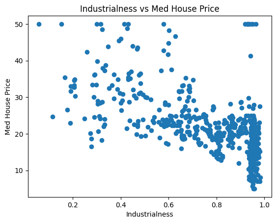
为了使示例简单,将仅使用两个功能:INDUS和RM。 这些和其他功能的解释可在数据页上找到。
1
2
3
4
5
6
7
# 获取bosten数据
data = boston_data;
# 仅仅处理INDUS和RM, 从data中选择所有行但只选择第3和第6列
x_input = data[:, [2,5]]
y_target = target;
# 标准化数据,使其拥有规则性
x_input = preprocessing.normalize(x_input)
1.1.3 可视化(Visualization)
1
2
3
4
5
6
7
8
9
10
11
12
# 对两个特征单独地画图
plt.title('Industrialness vs Med House Price')
plt.scatter(x_input[:, 0], y_target)
plt.xlabel('Industrialness')
plt.ylabel('Med House Price')
plt.show()
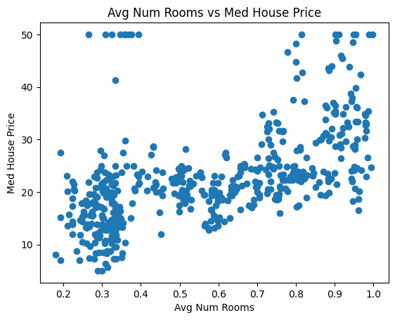
plt.title('Avg Num Rooms vs Med House Price')
plt.scatter(x_input[:, 1], y_target)
plt.xlabel('Avg Num Rooms')
plt.ylabel('Med House Price')
plt.show()
1.2 定义一个线性回归模型(Defining a Linear Regression Model)
线性回归模型为: \(f(x)=\mathbf{w}^\top \mathbf{x}+b=w_{1}x_{1}+w_{2}x_{2}+b,\)
np.dot(w, v) for vector dot product
np.dot(W, V) for matrix dot product
1
2
3
4
5
6
def linearmodel(w, b, x):
    '''
    Input: w 是权重, b 是截距, x 是d维的向量
    Output: 预测的输出
    '''
    return np.dot(w, x) + b
1
2
3
4
5
6
7
8
9
10
11
def linearmat_1(w, b, X):
    '''
    Input: w 是权重, b 是截距, X 是数据矩阵 (n x d)
    Output: 包含线性模型预测的向量
    '''
    # n 是训练例子的数量
    n = X.shape[0]
    t = np.zeros(n)
    for i in range(n):
        t[i] = linearmodel(w, b, X[i, :])
    return t
1.2.1 向量化(Vectorization)
1
2
3
4
5
6
7
def linearmat_2(w, X):
    '''
    linearmat_1的向量化.
    Input: w 是权重(包含截距), and X 数据矩阵 (n x (d+1)) (包含特征)
    Output:包含线性模型预测的向量
    '''
    return np.dot(X, w)
1.3 向量化和非向量化代码的速度比较(Comparing speed of the vectorized vs unvectorized code)
非向量化代码的时间
1
2
3
4
5
6
7
import time
w = np.array([1,1])
b = 1
t0 = time.time()
p1 = linearmat_1(w, b, x_input)
t1 = time.time()
print('the time for non-vectorized code is %s' % (t1 - t0))
向量化代码的时间
1
2
3
4
5
6
7
8
# 把截距添加到权重向量
wb = np.array([b, w[0], w[1]])
# 在输入矩阵中添加为1的参数(对应截距)
x_in = np.concatenate([np.ones([np.shape(x_input)[0], 1]), x_input], axis=1)
t0 = time.time()
p2 = linearmat_2(wb, x_in)
t1 = time.time()
print('the time for vectorized code is %s' % (t1 - t0))
1.4 定义损失函数(Defining the Cost Function)
\[C(\mathbf{y}, \mathbf{t}) = \frac{1}{2n}(\mathbf{y}-\mathbf{t})^\top (\mathbf{y}-\mathbf{t}).\]1
2
3
4
5
6
7
8
9
def cost(w, X, y):
'''
评估向量化方法的损失函数
输入 `X` 和输出 `y`, 在权重 `w`.
'''
residual = y - linearmat_2(w, X) # 获取差值
err = np.dot(residual, residual) / (2 * len(y))
return err
例如,假设的损失:
1
    cost(wb, x_in, y_target)
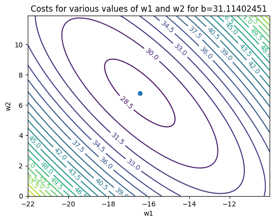
1.5 在权重空间画出损失(Plotting cost in weight space)
1
2
3
4
5
6
7
8
9
10
11
12
13
14
15
16
w1s = np.arange(-22, -10, 0.01)
w2s = np.arange(0, 12, 0.1)
b = 31.11402451
W1, W2 = np.meshgrid(w1s, w2s)
z_cost = np.zeros([len(w2s), len(w1s)])
for i in range(W1.shape[0]):
    for j in range(W1.shape[1]):
        w = np.array([b, W1[i, j], W2[i, j]])
        z_cost[i, j] = cost(w, x_in, y_target)
CS = plt.contour(W1, W2, z_cost,25)
plt.clabel(CS, inline=1, fontsize=10)
plt.title('Costs for various values of w1 and w2 for b=31.11402451')
plt.xlabel("w1")
plt.ylabel("w2")
plt.plot([-16.44307658], [6.79809451], 'o')
plt.show()
1.6 精确的解决方法(Exact Solution)
\[\mathbf{w}^*=(X^\top X)^{-1}X^\top y.\]1
2
3
4
5
6
7
8
9
10
11
12
13
14
def solve_exactly(X, y):
'''
精确解决线性回归(完全向量化)
给出 `X` - n x (d+1) 的输入矩阵
`y` - 目标输出
返回(d+1)维的最佳权重向量
'''
A = np.dot(X.T, X)
c = np.dot(X.T, y)
return np.dot(np.linalg.inv(A), c)
w_exact = solve_exactly(x_in, y_target)
print(w_exact)
2. 线性回归的梯度下降(Gradient Descent for Linear Regression)
2.1 Boston Housing的数据
2.1.1 导入库
1
2
3
4
5
6
import matplotlib
import numpy as np
import random
import warnings
import matplotlib.pyplot as plt
from sklearn import preprocessing   # for normalization
2.1.2 导入数据
1
2
3
4
5
6
7
8
9
10
11
12
13
14
import pandas as pd
import numpy as np
data_url = "https://lib.stat.cmu.edu/datasets/boston"
raw_df = pd.read_csv(data_url, sep="\s+", skiprows=22, header=None)
boston_data = np.hstack([raw_df.values[::2, :], raw_df.values[1::2, :2]])
target = raw_df.values[1::2, 2]

data = boston_data;
x_input = data  # a data matrix
y_target = target; # a vector for all outputs
# add a feature 1 to the dataset, then we do not need to consider the bias and weight separately
x_in = np.concatenate([np.ones([np.shape(x_input)[0], 1]), x_input], axis=1)
# we normalize the data so that each has regularity
x_in = preprocessing.normalize(x_in)
2.2 线性模型(Linear Model)
\[f(x)=\mathbf{w}^\top \mathbf{x}.\]1
2
3
4
5
6
7
def linearmat_2(w, X):
'''
linearmat_1的向量化.
Input: w 是权重(包含截距), and X 数据矩阵 (n x (d+1)) (包含特征)
Output:包含线性模型预测的向量
'''
return np.dot(X, w)
2.3 损失函数(Cost Function)
\[C(\mathbf{y}, \mathbf{t}) = \frac{1}{2n}(\mathbf{y}-\mathbf{t})^\top (\mathbf{y}-\mathbf{t}).\]1
2
3
4
5
6
7
8
9
def cost(w, X, y):
'''
评估向量化方法的损失函数
输入 `X` 和输出 `y`, 在权重 `w`.
'''
residual = y - linearmat_2(w, X) # 获取差值
err = np.dot(residual, residual) / (2 * len(y))
return err
2.4 梯度计算(Gradient Computation)
\[\nabla C(\mathbf{w}) =\frac{1}{n}X^\top\big(X\mathbf{w}-\mathbf{y}\big)\]1
2
3
4
5
6
7
8
9
10
11
12
# 向量化梯度方程
def gradfn(weights, X, y):
'''
给出 `weights` - 当前的对权重的猜想
`X` - (N,d+1)的包含特征`1`的输入特征矩阵
`y` - 目标y值
返回当前数值估计的权重梯度
'''
y_pred = np.dot(X, weights)
error = y_pred - y
return np.dot(X.T, error) / len(y)
2.5 梯度下降(Gradient Descent)
\[\mathbf{w}^{(t+1)} \leftarrow \mathbf{w}^{(t)} - \eta\nabla C(\mathbf{w}^{(t)})\]1
2
3
4
5
6
7
8
9
10
11
12
13
14
15
16
17
18
19
20
21
22
23
24
25
26
27
28
29
30
31
32
33
34
def solve_via_gradient_descent(X, y, print_every=100,
niter=5000, eta=1):
'''
给出 `X` - (N,D)的输入特征矩阵
`y` - 目标y值
`print_every` - 每'print_every' 迭代报告一次性能
`niter` - 迭代数量的限制
`eta` - 学习率
用梯度下降解决线性回归
返回
`w` - 在`niter`次迭代之后的权重
`idx_res` - 迭代的索引
`err_res` - 迭代的索引对应的损失值
'''
N, D = np.shape(X)
# 初始化所有的权重为0
w = np.zeros([D])
idx_res = []
err_res = []
for k in range(niter):
# 计算梯度
dw = gradfn(w, X, y)
# 梯度下降
w = w - eta * dw
# 每print_every迭代报告一次
if k % print_every == print_every - 1:
t_cost = cost(w, X, y)
print('error after %d iteration: %s' % (k, t_cost))
idx_res.append(k)
err_res.append(t_cost)
return w, idx_res, err_res
w_gd, idx_gd, err_gd = solve_via_gradient_descent( X=x_in, y=y_target)
Output(partial):
1
2
3
4
5
6
7
8
9
error after 2199 iteration: 26.616940808457816
error after 2299 iteration: 26.475493515509722
error after 2399 iteration: 26.33686272884545
error after 2499 iteration: 26.20095757351077
...
error after 4699 iteration: 23.78096067719028
error after 4799 iteration: 23.692775341901584
error after 4899 iteration: 23.606193772224405
error after 4999 iteration: 23.521184465124133
2.6 小批量梯度下降(Minibatch Grident Descent)
\(C(\mathbf{w})=\frac{1}{n}\sum_{i=1}^nC_i(\mathbf{w}),\) where $C_i(\mathbf{w})$ is the loss of the model $\mathbf{w}$ on the $i$-th example. In our Boston House Price prediction problem, $C_i$ takes the form $C_i(\mathbf{w})=\frac{1}{2}(\mathbf{w}^\top\mathbf{x}^{(i)}-y^{(i)})^2$.
1
2
3
4
5
6
7
8
9
10
11
12
13
14
15
16
17
18
19
20
21
22
23
24
25
26
27
28
29
30
31
32
33
34
35
36
def solve_via_minibatch(X, y, print_every=100,
                               niter=5000, eta=1, batch_size=50):
    '''
    求解具有 Nesterov 动量的线性回归权重。
    给出  `X` - (N,D)的输入特征矩阵
          `y` - 目标y值
          `print_every` - 每'print_every' 迭代报告一次性能
          `niter` - 迭代数量的限制
          `eta` - 学习率
          `batch_size` - 小批量的大小
    返回
        `w` - 在`niter`次迭代之后的权重
        `idx_res` - 迭代的索引
        `err_res` - 迭代的索引对应的损失值
    '''
    N, D = np.shape(X)
    # 初始化所有的权重为0
    w = np.zeros([D])
    idx_res = []
    err_res = []
    tset = list(range(N))
    for k in range(niter):
        idx = random.sample(tset, batch_size)
        #sample batch of data
        sample_X = X[idx, :]
        sample_y = y[idx]
        dw = gradfn(w, sample_X, sample_y)
        w = w - eta * dw
        if k % print_every == print_every - 1:
            t_cost = cost(w, X, y)
            print('error after %d iteration: %s' % (k, t_cost))
            idx_res.append(k)
            err_res.append(t_cost)
    return w, idx_res, err_res

w_batch, idx_batch, err_batch = solve_via_minibatch( X=x_in, y=y_target)
Output(partial):
1
2
3
4
5
6
7
8
9
error after 2199 iteration: 26.693266124289604
error after 2299 iteration: 26.467262454186802
error after 2399 iteration: 27.126877660242872
error after 2499 iteration: 26.318343441629153
...
error after 4699 iteration: 24.030476040027352
error after 4799 iteration: 23.87462298591681
error after 4899 iteration: 23.6754448557431
error after 4999 iteration: 23.54132978738581
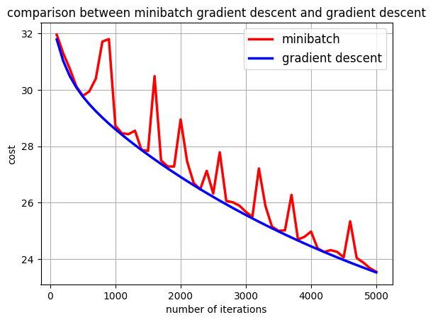
2.7 小批量梯度下降和梯度下降的比较(Comparison between Minibatch Gradient Descent and Gradient Descent)
1
2
3
4
5
6
7
8
plt.plot(idx_batch, err_batch, color="red", linewidth=2.5, linestyle="-", label="minibatch")
plt.plot(idx_gd, err_gd, color="blue", linewidth=2.5, linestyle="-", label="gradient descent")
plt.legend(loc='upper right', prop={'size': 12})
plt.title('comparison between minibatch gradient descent and gradient descent')
plt.xlabel("number of iterations")
plt.ylabel("cost")
plt.grid()
plt.show()
3. 感知器(Perceptron)
3.1 导入库
1
2
3
4
import numpy as np
import random
import matplotlib.pyplot as plt
from sklearn.metrics import accuracy_score
3.2 数据生成(Data Generation)
1
2
3
4
5
6
7
8
9
10
11
12
13
14
# `no_points`:表示要生成的数据点的数量。
def generate_data(no_points):
    # 创建一个形状为 (no_points, 2) 的零矩阵
    X = np.zeros(shape=(no_points, 2))
    # 创建一个长度为 no_points 的零向量
    Y = np.zeros(shape=no_points)
    for ii in range(no_points):
        X[ii, 0] = random.randint(0,20)
        X[ii, 1] = random.randint(0,20)
        if X[ii, 0]+X[ii, 1] > 20:
            Y[ii] = 1
        else:
            Y[ii] = -1
    return X, Y
3.3 类(Class)
1
2
3
4
class Person():
  def __init__(self, name, age):
    self.name = name
    self.age = age
1
2
3
4
5
6
7
8
p1 = Person("John", 36)

print(p1.name)
print(p1.age)
'''
John
36
'''
1
2
3
4
5
6
7
8
9
10
11
12
13
14
15
class Person():

  def __init__(self, name, age):
    self.name = name
    self.age = age

  def myfunc(self):
    print("Hello my name is " + self.name)

p1 = Person("John", 36)
p1.myfunc()

'''
Hello my name is John
'''
3.4 感知器逻辑(Perceptron Algorithm)
3.4.1 感知器(Perceptron)
\[\mathbf{x}\mapsto \text{sgn}(\mathbf{w}^\top\mathbf{x}+b)\]3.4.2 感知器逻辑(Perceptron Algorithm)
\[y(b+y+(\mathbf{w}+y\mathbf{x})^\top\mathbf{x})=yb+y\mathbf{w}^\top\mathbf{x}+y^2+y^2\mathbf{x}^\top\mathbf{x}> y(b+\mathbf{w}^\top\mathbf{x}).\]1
2
3
4
5
6
7
8
9
10
11
12
13
14
15
16
17
18
19
20
21
22
23
24
25
26
27
28
29
30
31
32
33
34
35
36
37
38
39
40
41
42
43
44
45
46
47
48
49
50
51
52
53
54
55
56
57
58
59
60
61
62
63
64
65
66
67
68
69
70
71
72
73
74
75
76
77
78
79
80
81
82
83
84
85
86
87
class Perceptron():
"""
Class for performing Perceptron.
X is the input array with n rows (no_examples) and d columns (no_features)
Y is a vector containing elements which indicate the class
(1 for positive class, -1 for negative class)
w is the weight vector (d dimensional vector)
b is the bias value
"""
def __init__(self, b = 0, max_iter = 1000):
# 最大迭代次数
self.max_iter = max_iter
# 权重
self.w = []
# 截距/偏置
self.b = 0
self.no_examples = 0
self.no_features = 0
def train(self, X, Y):
'''
This function applies the perceptron algorithm to train a model w based on X and Y.
It changes both w and b of the class.
'''
# we set the number of examples and the number of features according to the matrix X
self.no_examples, self.no_features = np.shape(X)
# we initialize the weight vector as the zero vector
self.w = np.zeros(self.no_features)
# we only run a limited number of iterations
for ii in range(0, self.max_iter):
# at the begining of each iteration, we set the w_updated to be false (meaning we have not yet found misclassified example)
w_updated = False
# we traverse all the training examples
for jj in range(0, self.no_examples):
# we compute the predicted value and assign it to the variable a
a = self.b + np.dot(self.w, X[jj])
# if we find a misclassified example
if Y[jj] * a <= 0:
# we set w_updated = true as we have found a misclassified example at this iteration
w_updated = True
# we now update w and b
self.w += Y[jj] * X[jj]
self.b += Y[jj]
# if we do not find any misclassified example, we can return the model
if not w_updated:
print("Convergence reached in %i iterations." % ii)
break
# after finishing the iterations we can still find a misclassified example
if w_updated:
print(
"""
WARNING: convergence not reached in %i iterations.
Either dataset is not linearly separable,
or max_iter should be increased
""" % self.max_iter
)
def classify_element(self, x_elem):
'''
This function returns the predicted label of the perceptron on an input x_elem
Input:
x_elem: an input feature vector
Output:
return the predictred label of the model (indicated by w and b) on x_elem
'''
return np.sign(self.b + np.dot(self.w, x_elem))
# To do: insert your code to complete the definition of the function classify a data matrix (n examples)
def classify(self, X):
'''
This function returns the predicted labels of the perceptron on an input matrix X
Input:
X: a data matrix with n rows (no_examples) and d columns (no_features)
Output:
return the vector. i-th entry is the predicted label on the i-th example
'''
# predicted_Y = []
# for ii in range(np.shape(X)[0]):
# # we predict the label and add the label to the output vector
# y_elem = self.classify_element(X[ii])
# predicted_Y.append(y_elem)
# # we return the output vector
# vectorization
out = np.dot(X, self.w)
predicted_Y = np.sign(out + self.b)
return predicted_Y
3.5 实验(Experiments)
3.5.1 数据生成(Data Generation)
1
X, Y = generate_data(100)
3.5.2 数据集的可视化(Visualization of the dataset)
1
2
3
4
5
6
idx_pos = [i for i in np.arange(100) if Y[i]==1]
idx_neg = [i for i in np.arange(100) if Y[i]==-1]
# make a scatter plot
plt.scatter(X[idx_pos, 0], X[idx_pos, 1], color='blue')
plt.scatter(X[idx_neg, 0], X[idx_neg, 1], color='red')
plt.show()

3.5.3 训练(Train)
1
2
3
4
5
6
7
# Create an instance p
p = Perceptron()
# applies the train algorithm to (X,Y) and sets the weight vector and bias
p.train(X, Y)
predicted_Y = p.classify(X)
acc_tr = accuracy_score(predicted_Y, Y)
print(acc_tr)
3.5.4 测试(Test)
1
2
3
4
5
# we first generate a new dataset
X_test, Y_test = generate_data(100)
predicted_Y_test = p.classify(X_test)
acc = accuracy_score(Y_test, predicted_Y_test)
print(acc)
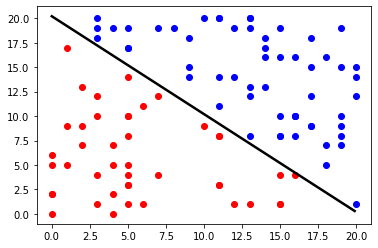
3.5.5 感知器的可视化(Visulization of the perceptron)
1
2
3
4
5
6
7
8
9
10
11
12
13
14
# we get an array of the first feature
x1 = np.arange(0, 20, 0.1)
# bias
b = p.b
# weight vector
w = p.w
# we now use list comprehension to generate the array of the second feature

x2 = [(-b-w[0]*x)/w[1] for x in x1]
plt.scatter(X[idx_pos, 0], X[idx_pos, 1], color='blue')
plt.scatter(X[idx_neg, 0], X[idx_neg, 1], color='red')
# plot the hyperplane corresponding to the perceptron
plt.plot(x1, x2, color="black", linewidth=2.5, linestyle="-")
plt.show()
4. 卷积神经网络(Convolutional Neural Network)
4.1 训练一个图像分类器(Training an image classifier)
- 加载并且用
torchvision标准化 CIFAR10 训练和测试数据集 - 定义一个卷积神经网络
- 定义一个损失函数
- 在训练集上训练网络
- 在测试集上测试网络
4.2 加载并且标准化CIFAR10(Load and normalize CIFAR10)
1
2
3
4
5
6
7
8
9
10
11
12
13
14
15
16
17
18
19
20
21
22
23
24
25
import torch
import torchvision
import torchvision.transforms as transforms

device = torch.device("cuda:0" if torch.cuda.is_available() else "cpu")
print(f"The current device is {device}")

transform = transforms.Compose(
[transforms.ToTensor(),
 transforms.Normalize((0.5, 0.5, 0.5), (0.5, 0.5, 0.5))])

batch_size = 4

trainset = torchvision.datasets.CIFAR10(root='./data', train=True,
                                            download=True, transform=transform)
trainloader = torch.utils.data.DataLoader(trainset, batch_size=batch_size,
                                              shuffle=True, num_workers=2)

testset = torchvision.datasets.CIFAR10(root='./data', train=False,
                                           download=True, transform=transform)
testloader = torch.utils.data.DataLoader(testset, batch_size=batch_size,
                                             shuffle=False, num_workers=2)

classes = ('plane', 'car', 'bird', 'cat',
           'deer', 'dog', 'frog', 'horse', 'ship', 'truck')
If running on Windows and you get a BrokenPipeError, try setting the num_worker of torch.utils.data.DataLoader() to 0
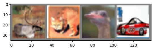
显示部分训练图像
1
2
3
4
5
6
7
8
9
10
11
12
13
14
15
16
17
18
19
20
21
import matplotlib.pyplot as plt
import numpy as np

# functions to show an image


def imshow(img):
    img = img / 2 + 0.5     # unnormalize
    npimg = img.numpy()
    plt.imshow(np.transpose(npimg, (1, 2, 0)))
    plt.show()


# get some random training images
dataiter = iter(trainloader)
images, labels = next(dataiter)

# show images
imshow(torchvision.utils.make_grid(images))
# print labels
print(' '.join('%5s' % classes[labels[j]] for j in range(batch_size)))
4.3 定义一个卷积神经网络(Define a Convolutional Neural Network)
1
2
3
4
5
6
7
8
9
10
11
12
13
14
15
16
17
18
19
20
21
22
23
24
25
26
27
28
29
30
import torch.nn as nn
import torch.nn.functional as F


class Net(nn.Module):
    def __init__(self):
        super().__init__()
        # 从3个输入通道到6个输出通道,使用5x5的卷积核
        self.conv1 = nn.Conv2d(3, 6, 5)
        # 使用2x2的窗口大小并且步长为2
        self.pool = nn.MaxPool2d(2, 2)
        # 从6个输入通道到16个输出通道,也使用5x5的卷积核
        self.conv2 = nn.Conv2d(6, 16, 5)
        # 16x5x5的张量展平为120个特征
        self.fc1 = nn.Linear(16 * 5 * 5, 120)
        self.fc2 = nn.Linear(120, 84)
        self.fc3 = nn.Linear(84, 10)

    def forward(self, x):
        # ReLU激活函数
        x = self.pool(F.relu(self.conv1(x)))
        x = self.pool(F.relu(self.conv2(x)))
        x = torch.flatten(x, 1) # flatten all dimensions except batch
        x = F.relu(self.fc1(x))
        x = F.relu(self.fc2(x))
        x = self.fc3(x)
        return x


net = Net().to(device)
4.4 定义一个损失函数与优化器(Define a Loss function and optimizer)
1
2
3
4
5
6
7
# 导入pytorch提供的优化算法
import torch.optim as optim

# 定义了交叉熵损失函数
criterion = nn.CrossEntropyLoss()
# 使用随机梯度下降(SGD)作为优化算法, 设置学习率为0.001, 设置动量为0.9。动量在SGD中用于加速训练并避免陷入局部最小值。
optimizer = optim.SGD(net.parameters(), lr=0.001, momentum=0.9)
4.5 训练网络(Train the network)
1
2
3
4
5
6
7
8
9
10
11
12
13
14
15
16
17
18
19
20
21
22
23
24
25
26
27
28
29
30
31
32
# 遍历整个数据集两次
for epoch in range(2):

    # 用于累积每个批次的损失,以便后续打印平均损失
    running_loss = 0.0
    for i, data in enumerate(trainloader, 0):
        # get the inputs; data is a list of [inputs, labels] and move them to
        #the current device
        inputs, labels = data
        inputs = inputs.to(device)
        labels = labels.to(device)

        # 在每次训练步骤之前,将模型中所有参数的梯度设置为零
        optimizer.zero_grad()

        # forward + backward + optimize
        outputs = net(inputs)
        loss = criterion(outputs, labels)
        loss.backward()
        optimizer.step()

        # print statistics - epoch and loss
        running_loss += loss.item()
        if i % 2000 == 1999:    # print every 2000 mini-batches
            print('[%d, %5d] loss: %.3f' %
                  (epoch + 1, i + 1, running_loss / 2000))
            running_loss = 0.0

print('Finished Training')

PATH = './cifar_net.pth'
torch.save(net.state_dict(), PATH)
4.6 在测试数据上测试网络(Test the network on the test data)
选择一批测试数据并显示
1
2
3
4
5
6
dataiter = iter(testloader)
images, labels = next(dataiter) #Selects a mini-batch and its labels

# print images
imshow(torchvision.utils.make_grid(images))
print('GroundTruth: ', ' '.join('%5s' % classes[labels[j]] for j in range(4)))
加载预先保存的模型参数
1
2
net = Net()
net.load_state_dict(torch.load(PATH))
在单批数据上预测
1
2
3
4
images = images.to(device)
labels = labels.to(device)
net = net.to(device)
outputs = net(images)
获取预测结果:
1
2
3
4
_, predicted = torch.max(outputs, 1) #Returns a tuple (max,max indicies), we only need the max indicies.

print('Predicted: ', ' '.join('%5s' % classes[predicted[j]]
                              for j in range(4)))
评估整体测试集的准确性:
1
2
3
4
5
6
7
8
9
10
11
12
13
14
15
16
17
18
19
correct = 0
total = 0
# since we're not training, we don't need to calculate the gradients for our outputs
with torch.no_grad():
    for data in testloader:
        images, labels = data
        images = images.to(device)
        labels = labels.to(device)

        # calculate outputs by running images through the network
        outputs = net(images)

        # the class with the highest energy is what we choose as prediction
        _, predicted = torch.max(outputs.data, 1)
        total += labels.size(0)
        correct += (predicted == labels).sum().item()

print('Accuracy of the network on the 10000 test images: %d %%' % (
    100 * correct / total))
评估每个类的准确性:
1
2
3
4
5
6
7
8
9
10
11
12
13
14
15
16
17
18
19
20
21
22
23
24
25
# prepare to count predictions for each class
correct_pred = {classname: 0 for classname in classes}
total_pred = {classname: 0 for classname in classes}

# again no gradients needed
with torch.no_grad():
    for data in testloader:
        images, labels = data
        images = images.to(device)
        labels = labels.to(device)

        outputs = net(images)
        _, predictions = torch.max(outputs, 1)
        # collect the correct predictions for each class
        for label, prediction in zip(labels, predictions):
            if label == prediction:
                correct_pred[classes[label]] += 1
            total_pred[classes[label]] += 1


# print accuracy for each class
for classname, correct_count in correct_pred.items():
    accuracy = 100 * float(correct_count) / total_pred[classname]
    print("Accuracy for class {:5s} is: {:.1f} %".format(classname,
                                                   accuracy))
5. 自动编码器(AutoEncoders)
5.1 加载和刷新MNIST(Loading and refreshing MNIST)
1
2
3
4
5
6
7
8
9
10
11
12
13
14
15
16
17
18
19
20
21
22
23
24
25
26
27
28
29
30
31
32
33
34
35
36
37
38
39
40
41
42
43
# -*- coding: utf-8 -*- 该文件使用UTF-8编码
# The below is for auto-reloading external modules after they are changed, such as those in ./utils.
# Issue: https://stackoverflow.com/questions/1907993/autoreload-of-modules-in-ipython

# Jupyter Notebook的特定命令,用于自动重新加载外部模块
%load_ext autoreload
%autoreload 2

# `numpy`库用于数组操作,`get_mnist`函数用于获取MNIST数据集
import numpy as np
from utils.data_utils import get_mnist # Helper function. Use it out of the box.

# 常量定义: 数据的存储位置和一个随机种子
DATA_DIR = './data/mnist' # Location we will keep the data.
SEED = 111111

# 使用get_mnist函数从指定的目录加载训练和测试数据。如果数据不在指定位置,它们将被下载
train_imgs, train_lbls = get_mnist(data_dir=DATA_DIR, train=True, download=True)
test_imgs, test_lbls = get_mnist(data_dir=DATA_DIR, train=False, download=True)

# 输出训练和测试数据的相关信息,如其类型、形状、数据类型以及类标签
print("[train_imgs] Type: ", type(train_imgs), "|| Shape:", train_imgs.shape, "|| Data type: ", train_imgs.dtype )
print("[train_lbls] Type: ", type(train_lbls), "|| Shape:", train_lbls.shape, "|| Data type: ", train_lbls.dtype )
print('Class labels in train = ', np.unique(train_lbls))

print("[test_imgs] Type: ", type(test_imgs), "|| Shape:", test_imgs.shape, " || Data type: ", test_imgs.dtype )
print("[test_lbls] Type: ", type(test_lbls), "|| Shape:", test_lbls.shape, " || Data type: ", test_lbls.dtype )
print('Class labels in test = ', np.unique(test_lbls))

# 定义了一些与数据集相关的其他常量,如训练图像的数量、图像的高度、图像的宽度和类别的数量
N_tr_imgs = train_imgs.shape[0] # N hereafter. Number of training images in database.
H_height = train_imgs.shape[1] # H hereafter
W_width = train_imgs.shape[2] # W hereafter
C_classes = len(np.unique(train_lbls)) # C hereafter

'''
[train_imgs] Type:  <class 'numpy.ndarray'> || Shape: (60000, 28, 28) || Data type:  uint8
[train_lbls] Type:  <class 'numpy.ndarray'> || Shape: (60000,) || Data type:  int16
Class labels in train =  [0 1 2 3 4 5 6 7 8 9]
[test_imgs] Type:  <class 'numpy.ndarray'> || Shape: (10000, 28, 28)  || Data type:  uint8
[test_lbls] Type:  <class 'numpy.ndarray'> || Shape: (10000,)  || Data type:  int16
Class labels in test =  [0 1 2 3 4 5 6 7 8 9]
'''
1
2
3
4
5
6
7
8
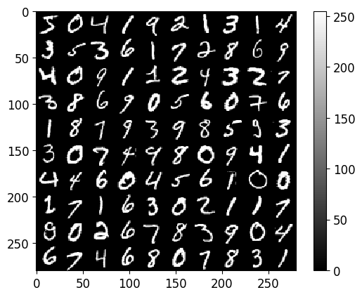
# Jupyter Notebook特定的命令,保证matplotlib库生成的图像都直接在Notebook内显示
%matplotlib inline
# 导入库,将多个图像绘制在一个网格上
from utils.plotting import plot_grid_of_images # Helper functions, use out of the box.
# 绘制了train_imgs中的前100个图像。图像被组织成一个10x10的网格,每行显示10个图像
plot_grid_of_images(train_imgs[0:100], n_imgs_per_row=10)
5.2 数据预处理(Data pre-processing)
5.2.1 将标签的表示更改为长度 C=10 的 one-hot 向量(Change representation of labels to one-hot vectors of length C=10)
1
2
3
4
5
6
7
8
9
10
11
12
13
14
15
# 为训练和测试标签初始化一个全为0的矩阵。每个标签都将在对应的独热编码向量中有一个值为1的元素
# 对于每个训练标签,我们找到其对应的独热编码向量中应该为1的位置,并将该位置的值设置为1
train_lbls_onehot = np.zeros(shape=(train_lbls.shape[0], C_classes ) )
train_lbls_onehot[ np.arange(train_lbls_onehot.shape[0]), train_lbls ] = 1
test_lbls_onehot = np.zeros(shape=(test_lbls.shape[0], C_classes ) )
test_lbls_onehot[ np.arange(test_lbls_onehot.shape[0]), test_lbls ] = 1

# 打印了转换前后标签的类型、形状和数据类型
print("BEFORE: [train_lbls]        Type: ", type(train_lbls), "|| Shape:", train_lbls.shape, " || Data type: ", train_lbls.dtype )
print("AFTER : [train_lbls_onehot] Type: ", type(train_lbls_onehot), "|| Shape:", train_lbls_onehot.shape, " || Data type: ", train_lbls_onehot.dtype )

'''
BEFORE: [train_lbls]        Type:  <class 'numpy.ndarray'> || Shape: (60000,)  || Data type:  int16
AFTER : [train_lbls_onehot] Type:  <class 'numpy.ndarray'> || Shape: (60000, 10)  || Data type:  float64
'''
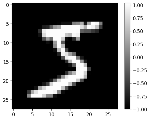
5.2.2 重新缩放图像强度,从 [0,255] 到 [-1, +1](Re-scale image intensities, from [0,255] to [-1, +1])
1
2
3
4
5
6
7
8
9
10
11
12
13
14
15
16
17
18
19
20
21
22
# This commonly facilitates learning:
# A zero-centered signal with small magnitude allows avoiding exploding/vanishing problems easier.
from utils.data_utils import normalize_int_whole_database # Helper function. Use out of the box.
# 图像的强度值被归一化到了[-1, +1]的范围
train_imgs = normalize_int_whole_database(train_imgs, norm_type="minus_1_to_1")
test_imgs = normalize_int_whole_database(test_imgs, norm_type="minus_1_to_1")

# Lets plot one image.
from utils.plotting import plot_image # Helper function, use out of the box.
index = 0  # Try any, up to 60000
print("Plotting image of index: [", index, "]")
print("Class label for this image is: ", train_lbls[index])
print("One-hot label representation: [", train_lbls_onehot[index], "]")
plot_image(train_imgs[index])
# Notice the magnitude of intensities. Black is now negative and white is positive float.
# Compare with intensities of figure further above.

'''
Plotting image of index: [ 0 ]
Class label for this image is:  5
One-hot label representation: [ [0. 0. 0. 0. 0. 1. 0. 0. 0. 0.] ]
'''
5.2.3 将图像从 2D 矩阵展平为 1D 向量。 MLP 将特征向量作为输入,而不是 2D 图像(Flatten the images, from 2D matrices to 1D vectors. MLPs take feature-vectors as input, not 2D images)
1
2
3
4
5
6
7
8
9
10
11
12
13
# 展平图像数据:
#     将每张图像的像素展平成一个一维数组。这通常是在将图像数据输入到全连接神经网络之前所需要做的,因为全连接层需要一维的输入向量
train_imgs_flat = train_imgs.reshape([train_imgs.shape[0], -1]) # Preserve 1st dim (S = num Samples), flatten others.
test_imgs_flat = test_imgs.reshape([test_imgs.shape[0], -1])
print("Shape of numpy array holding the training database:")
print("Original : [N, H, W] = [", train_imgs.shape , "]")
print("Flattened: [N, H*W]  = [", train_imgs_flat.shape , "]")

'''
Shape of numpy array holding the training database:
Original : [N, H, W] = [ (60000, 28, 28) ]
Flattened: [N, H*W]  = [ (60000, 784) ]
'''
5.3 为了AE用SGD进行无监督训练(Unsupervised training with SGD for Auto-Encoders)
1
2
3
4
5
6
7
8
9
10
11
12
13
14
15
16
17
18
19
20
21
22
23
24
25
26
27
28
29
30
31
32
33
34
35
36
37
38
39
40
41
42
43
44
45
46
47
48
49
50
51
52
53
54
55
56
57
58
59
60
61
62
63
64
65
66
67
68
69
70
71
72
73
74
75
76
77
78
79
80
81
82
83
84
85
86
87
88
from utils.plotting import plot_train_progress_1, plot_grids_of_images # Use out of the box
# 从训练数据中随机抽取一个批次的图片
def get_random_batch(train_imgs, train_lbls, batch_size, rng):
# train_imgs: Images. Numpy array of shape [N, H, W]
# train_lbls: Labels of images. None, or Numpy array of shape [N, C_classes], one hot label for each image.
# batch_size: integer. Size that the batch should have.
####### Sample a random batch of images for training. Fill in the blanks (???) #########
indices = range(0, batch_size) # Remove this line after you fill-in and un-comment the below.
indices = rng.randint(low=0, high=train_imgs.shape[0], size=batch_size, dtype='int32')
#indices = rng.randint(low=??????, high=train_imgs.shape[???????], size=?????????, dtype='int32')
##############################################################################################
train_imgs_batch = train_imgs[indices]
if train_lbls is not None: # Enables function to be used both for supervised and unsupervised learning
train_lbls_batch = train_lbls[indices]
else:
train_lbls_batch = None
return [train_imgs_batch, train_lbls_batch]
def unsupervised_training_AE(net,
loss_func,
rng,
train_imgs_all,
batch_size,
learning_rate,
total_iters,
iters_per_recon_plot=-1):
# net: 自编码器网络对象 Instance of a model. See classes: Autoencoder, MLPClassifier, etc further below
# loss_func: 用于计算损失的函数 Function that computes the loss. See functions: reconstruction_loss or cross_entropy.
# rng: 随机数生成器对象 numpy random number generator
# train_imgs_all: 训练图像的完整集合 All the training images. Numpy array, shape [N_tr, H, W]
# batch_size: 每次迭代用于训练的图像数量 Size of the batch that should be processed per SGD iteration by a model.
# learning_rate: 优化器的学习率 self explanatory.
# total_iters: 训练总迭代次数 how many SGD iterations to perform.
# iters_per_recon_plot: 每隔多少迭代绘制一次重构图像,默认为-1,表示不绘制 Integer. Every that many iterations the model predicts training images ...
# ...and we plot their reconstruction. For visual observation of the results.
# 初始化一个空列表,用于存储训练过程中的损失值。
loss_values_to_plot = []
# 创建一个Adam优化器,用于更新网络 net 的参数。
optimizer = optim.Adam(net.params, lr=learning_rate) # Will use PyTorch's Adam optimizer out of the box
# 随机梯度下降(SGD)
for t in range(total_iters):
# Sample batch for this SGD iteration
x_imgs, _ = get_random_batch(train_imgs_all, None, batch_size, rng)
# Forward pass: 通过网络执行前向传播,获取重构的图像和编码的潜在表示。
x_pred, z_codes = net.forward_pass(x_imgs)
# Compute loss: 计算重构图像和原始图像之间的损失。
loss = loss_func(x_pred, x_imgs)
# Pytorch way
# 在每次梯度更新前清零累积的梯度。
optimizer.zero_grad()
# 执行反向传播,计算损失相对于网络参数的梯度。
_ = net.backward_pass(loss)
# 应用梯度更新网络参数。
optimizer.step()
# ==== Report training loss and accuracy ======
loss_np = loss if type(loss) is type(float) else loss.item() # Pytorch returns tensor. Cast to float
print("[iter:", t, "]: Training Loss: {0:.2f}".format(loss))
loss_values_to_plot.append(loss_np)
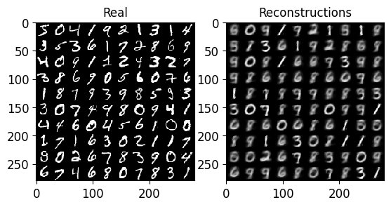
# =============== Every few iterations, show reconstructions ================#
if t==total_iters-1 or t%iters_per_recon_plot == 0:
# Reconstruct all images, to plot reconstructions.
x_pred_all, z_codes_all = net.forward_pass(train_imgs_all)
# Cast tensors to numpy arrays
x_pred_all_np = x_pred_all if type(x_pred_all) is np.ndarray else x_pred_all.detach().numpy()
# Predicted reconstructions have vector shape. Reshape them to original image shape.
train_imgs_resh = train_imgs_all.reshape([train_imgs_all.shape[0], H_height, W_width])
x_pred_all_np_resh = x_pred_all_np.reshape([train_imgs_all.shape[0], H_height, W_width])
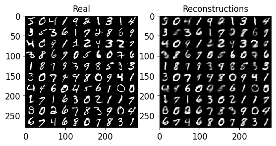
# Plot a few images, originals and predicted reconstructions.
plot_grids_of_images([train_imgs_resh[0:100], x_pred_all_np_resh[0:100]],
titles=["Real", "Reconstructions"],
n_imgs_per_row=10,
dynamically=True)
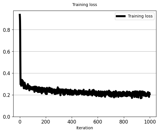
# In the end of the process, plot loss.
plot_train_progress_1(loss_values_to_plot, iters_per_point=1)
5.4 自动编码器(Auto-Encoder)
1
2
3
4
5
6
7
8
9
10
11
12
13
14
15
16
17
18
19
20
21
22
23
24
25
26
27
28
29
30
31
32
33
34
35
36
37
38
39
40
41
42
43
44
45
46
47
48
49
50
51
52
53
54
55
56
57
58
59
60
61
62
63
64
65
66
67
68
69
70
71
72
73
74
75
76
77
78
79
80
81
82
83
84
85
86
87
88
89
90
91
92
93
94
95
96
97
98
99
100
101
102
103
104
105
106
107
108
109
110
111
112
113
114
115
116
117
118
119
120
121
122
123
124
125
126
127
128
129
130
131
132
133
134
135
136
137
138
139
140
141
142
143
144
145
146
147
148
149
150
151
152
153
154
155
156
157
158
159
160
161
162
163
164
165
166
# -*- coding: utf-8 -*-
import torch
import torch.optim as optim
import torch.nn as nn

# 定义了一个基本的神经网络结构和反向传播
class Network():

    def backward_pass(self, loss):
        # Performs back propagation and computes gradients
        # With PyTorch, we do not need to compute gradients analytically for parameters were requires_grads=True,
        # Calling loss.backward(), torch's Autograd automatically computes grads of loss wrt each parameter p,...
        # ... and **puts them in p.grad**. Return them in a list.
        loss.backward()
        grads = [param.grad for param in self.params]
        return grads

# 定义了一个四层的自编码器。网络由输入层、编码器隐藏层、瓶颈层、解码器隐藏层和输出层组成
class Autoencoder(Network):
    def __init__(self, rng, D_in, D_hid_enc, D_bottleneck, D_hid_dec):
        # Construct and initialize network parameters
        D_in = D_in # Dimension of input feature-vectors. Length of a vectorised image.
        D_hid_1 = D_hid_enc # Dimension of Encoder's hidden layer
        D_hid_2 = D_bottleneck
        D_hid_3 = D_hid_dec  # Dimension of Decoder's hidden layer
        D_out = D_in # Dimension of Output layer.

        self.D_bottleneck = D_bottleneck  # Keep track of it, we will need it.

        ##### TODO: Initialize the Auto-Encoder's parameters. Also see forward_pass(...)) ########
        # Dimensions of parameter tensors are (number of neurons + 1) per layer, to account for +1 bias.
        # 初始化权重的值, 根据正态随机分布
        w1_init = rng.normal(loc=0.0, scale=0.01, size=(D_in+1, D_hid_1))
        w2_init = rng.normal(loc=0.0, scale=0.01, size=(D_hid_1+1, D_hid_2))
        w3_init = rng.normal(loc=0.0, scale=0.01, size=(D_hid_2+1, D_hid_3))
        w4_init = rng.normal(loc=0.0, scale=0.01, size=(D_hid_3+1, D_out))
        # Pytorch tensors, parameters of the model
        # Use the above numpy arrays as of random floats as initialization for the Pytorch weights.
        # 权重被转换为tensor张量
        w1 = torch.tensor(w1_init, dtype=torch.float, requires_grad=True)
        w2 = torch.tensor(w2_init, dtype=torch.float, requires_grad=True)
        w3 = torch.tensor(w3_init, dtype=torch.float, requires_grad=True)
        w4 = torch.tensor(w4_init, dtype=torch.float, requires_grad=True)
        # Keep track of all trainable parameters:
        self.params = [w1, w2, w3, w4]
        ###########################################################################

    # 定义了输入如何通过自编码器的各层进行处理。它对编码器和解码器隐藏层使用ReLU激活函数(preact),并对输出层使用tanh激活函数
    def forward_pass(self, batch_imgs):
        # Get parameters
        [w1, w2, w3, w4] = self.params

        # 将输入数据转换为torch张量
        batch_imgs_t = torch.tensor(batch_imgs, dtype=torch.float)  # Makes pytorch array to pytorch tensor.

        # 添加bias单元
        unary_feature_for_bias = torch.ones(size=(batch_imgs.shape[0], 1)) # [N, 1] column vector.
        x = torch.cat((batch_imgs_t, unary_feature_for_bias), dim=1) # Extra feature=1 for bias.

        #### TODO: Implement the operations at each layer #####
        # Layer 1
        h1_preact = x.mm(w1) # 计算预激活值
        h1_act = h1_preact.clamp(min=0) # 应用ReLU激活函数
        # Layer 2 (bottleneck):
        h1_ext = torch.cat((h1_act, unary_feature_for_bias), dim=1) # 添加bias单元到隐藏层1
        h2_preact = h1_ext.mm(w2) # 计算预激活值
        h2_act = h2_preact.clamp(min=0) # 应用ReLU激活函数
        # Layer 3:
        h2_ext = torch.cat((h2_act, unary_feature_for_bias), dim=1) # 添加bias单元到隐藏层2
        h3_preact = h2_ext.mm(w3) # 计算预激活值
        h3_act = h3_preact.clamp(min=0) # 应用ReLU激活函数
        # Layer 4 (output):
        h3_ext = torch.cat((h3_act, unary_feature_for_bias), dim=1) # 添加bias单元到隐藏层3
        h4_preact = h3_ext.mm(w4) # 计算预激活值
        h4_act = torch.tanh(h4_preact) # 应用tanh激活函数
        # Output layer
        x_pred = h4_act
        #######################################################

        ### TODO: Get bottleneck's activations ######
        # Bottleneck actications
        acts_bottleneck = h2_act
        #############################################

        return (x_pred, acts_bottleneck)

# 计算重建图像与原始图像之间的均方误差。这个损失在训练过程中用于调整网络的权重
def reconstruction_loss(x_pred, x_real, eps=1e-7):
    # Cross entropy: See Lecture 5, slide 19.
    # x_pred: [N, D_out] Prediction returned by forward_pass. Numpy array of shape [N, D_out]
    # x_real: [N, D_in]

    # If number array is given, change it to a Torch tensor.
    x_pred = torch.tensor(x_pred, dtype=torch.float) if type(x_pred) is np.ndarray else x_pred
    x_real = torch.tensor(x_real, dtype=torch.float) if type(x_real) is np.ndarray else x_real

    ######## TODO: Complete the calculation of Reconstruction loss for each sample ###########
    loss_recon = torch.mean(torch.square(x_pred - x_real), dim=1)
    # NOTE: Notice a difference from theory in Lecture: In implementations, we often calculate...
    # the *mean* square error over output's dimensions, rather than the *sum* as often shown in theory.
    # This makes the loss independent of the dimensionality of the input/output, so it can be used
    # without any change for different architectures and image sizes.
    # Otherwise we'd have to adapt the Learning rate whenever we use a network for different image sizes
    # to account for the change of the loss's scale.
    ##########################################################################################

    cost = torch.mean(loss_recon, dim=0) # Expectation of loss: Mean over samples (axis=0).
    return cost


# Create the network
rng = np.random.RandomState(seed=SEED)
autoencoder_thin = Autoencoder(rng=rng,
                               D_in=H_height*W_width,
                               D_hid_enc=256,
                               D_bottleneck=2,
                               D_hid_dec=256)
# Start training
# 定义了自编码器的训练循环。过程包括:
#       随机抽取图像批次。
#       通过自编码器处理图像以获得重构的输出。
#       计算重构和原始图像之间的损失。
#       反向传播来更新网络的权重。
#       可选择地每隔几次迭代绘制重构的图像进行可视化。
unsupervised_training_AE(autoencoder_thin,
                         reconstruction_loss,
                         rng,
                         train_imgs_flat,
                         batch_size=40,
                         learning_rate=3e-3,
                         total_iters=1000,
                         iters_per_recon_plot=50)

'''
[iter: 0 ]: Training Loss: 0.94
[iter: 1 ]: Training Loss: 0.92
[iter: 2 ]: Training Loss: 0.88
[iter: 3 ]: Training Loss: 0.78
[iter: 4 ]: Training Loss: 0.60
[iter: 5 ]: Training Loss: 0.42
[iter: 6 ]: Training Loss: 0.30
[iter: 7 ]: Training Loss: 0.33
[iter: 8 ]: Training Loss: 0.31
[iter: 9 ]: Training Loss: 0.32
[iter: 10 ]: Training Loss: 0.32
[iter: 11 ]: Training Loss: 0.28
[iter: 12 ]: Training Loss: 0.32
[iter: 13 ]: Training Loss: 0.32
[iter: 14 ]: Training Loss: 0.32
[iter: 15 ]: Training Loss: 0.31
[iter: 16 ]: Training Loss: 0.32
[iter: 17 ]: Training Loss: 0.34
[iter: 18 ]: Training Loss: 0.33
[iter: 19 ]: Training Loss: 0.32
[iter: 20 ]: Training Loss: 0.29
[iter: 21 ]: Training Loss: 0.30
[iter: 22 ]: Training Loss: 0.31
[iter: 23 ]: Training Loss: 0.33
[iter: 24 ]: Training Loss: 0.32
[iter: 25 ]: Training Loss: 0.29
...
[iter: 47 ]: Training Loss: 0.26
[iter: 48 ]: Training Loss: 0.27
[iter: 49 ]: Training Loss: 0.28
[iter: 50 ]: Training Loss: 0.27
'''
5.5 对潜在(瓶颈)表示中的所有训练样本进行编码(Encode all training samples in the latent (bottleneck) representation)
1
2
3
4
5
6
7
8
9
10
11
12
13
14
15
16
17
18
19
20
21
22
23
24
25
26
27
28
29
30
31
32
33
34
35
36
37
38
39
40
41
42
43
44
45
46
47
48
49
50
51
52
53
54
55
56
57
58
59
60
61
62
63
64
65
66
67
68
69
70
import matplotlib.pyplot as plt
# 接受的参数包括一个网络、一组扁平化的图像、标签、批处理大小、总迭代次数和一个布尔值决定是否绘制二维嵌入
def encode_and_get_min_max_z(net,
imgs_flat,
lbls,
batch_size,
total_iterations=None,
plot_2d_embedding=True):
# This function encodes images, plots the first 2 dimensions of the codes in a plot, and finally...
# ... returns the minimum and maximum values of the codes for each dimensions of Z.
# ... We will use this at a layer task.
# Arguments:
# imgs_flat: Numpy array of shape [Number of images, H * W]
# lbls: Numpy array of shape [number of images], with 1 integer per image. The integer is the class (digit).
# total_iterations: How many batches to encode. We will use this so that we dont encode and plot ...
# ... the whoooole training database, because the plot will get cluttered with 60000 points.
# Returns:
# min_z: numpy array, vector with [dimensions-of-z] elements. Minimum value per dimension of z.
# max_z: numpy array, vector with [dimensions-of-z] elements. Maximum value per dimension of z.
# If total iterations is None, the function will just iterate over all data, by breaking them into batches.
if total_iterations is None:
total_iterations = (train_imgs_flat.shape[0] - 1) // batch_size + 1
z_codes_all = []
lbls_all = []
for t in range(total_iterations):
# Sample batch for this SGD iteration
x_batch = imgs_flat[t*batch_size: (t+1)*batch_size]
lbls_batch = lbls[t*batch_size: (t+1)*batch_size]
# Forward pass:执行前向传递得到预测的图像和编码值
x_pred, z_codes = net.forward_pass(x_batch)
# 如果编码值不是numpy数组,则将其转换为numpy数组
z_codes_np = z_codes if type(z_codes) is np.ndarray else z_codes.detach().numpy()
# 将编码值和标签存储在列表中
z_codes_all.append(z_codes_np) # List of np.arrays
lbls_all.append(lbls_batch)
z_codes_all = np.concatenate(z_codes_all) # Make list of arrays in one array by concatenating along dim=0 (image index)
lbls_all = np.concatenate(lbls_all)
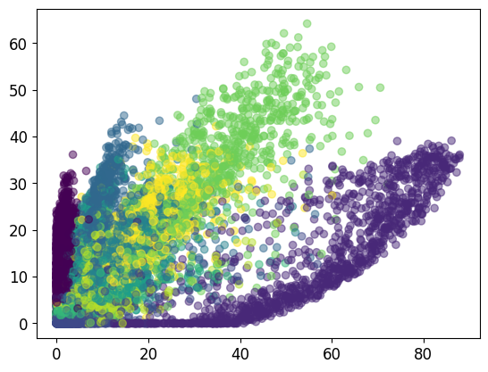
if plot_2d_embedding:
# Plot the codes with different color per class in a scatter plot:
plt.scatter(z_codes_all[:,0], z_codes_all[:,1], c=lbls_all, alpha=0.5) # Plot the first 2 dimensions.
plt.show()
# 计算并返回编码值的每个维度的最小和最大值
min_z = np.min(z_codes_all, axis=0) # min and max for each dimension of z, over all samples.
max_z = np.max(z_codes_all, axis=0) # Numpy array (vector) of shape [number of z dimensions]
return min_z, max_z
# Encode training samples, and get the min and max values of the z codes (for each dimension)
min_z, max_z = encode_and_get_min_max_z(autoencoder_thin,
train_imgs_flat,
train_lbls,
batch_size=100,
total_iterations=100)
print("Min Z value per dimension of bottleneck:", min_z)
print("Max Z value per dimension of bottleneck:", max_z)
'''
Min Z value per dimension of bottleneck: [0. 0.]
Max Z value per dimension of bottleneck: [87.92656 64.17436]
'''
5.6 用一个大的瓶颈层训练AE(Train an Auto-Encoder with a larger bottleneck layer)
1
2
3
4
5
6
7
8
9
10
11
12
13
14
15
16
17
18
19
20
21
22
23
24
25
26
27
28
29
30
31
32
33
34
35
# 这个任务的目标是检查一个更宽的自编码器如何进行训练,以及它的性能如何
# The below is a copy paste from Task 2.

# Create the network
rng = np.random.RandomState(seed=SEED)
autoencoder_wide = Autoencoder(rng=rng,
                               D_in=H_height*W_width,
                               D_hid_enc=256,
                               D_bottleneck=32,
                               D_hid_dec=256)
# Start training
unsupervised_training_AE(autoencoder_wide,
                         reconstruction_loss,
                         rng,
                         train_imgs_flat,
                         batch_size=40,
                         learning_rate=3e-3,
                         total_iters=1000,
                         iters_per_recon_plot=50)

'''
[iter: 968 ]: Training Loss: 0.10
[iter: 969 ]: Training Loss: 0.11
[iter: 970 ]: Training Loss: 0.10
[iter: 971 ]: Training Loss: 0.12
[iter: 972 ]: Training Loss: 0.11
[iter: 973 ]: Training Loss: 0.10
[iter: 974 ]: Training Loss: 0.12
[iter: 975 ]: Training Loss: 0.12
...
[iter: 996 ]: Training Loss: 0.11
[iter: 997 ]: Training Loss: 0.11
[iter: 998 ]: Training Loss: 0.11
[iter: 999 ]: Training Loss: 0.11
'''

5.7 基本自动编码器是否适合合成新数据?(Is basic Auto-Encoder appropriate for synthesizing new data?)
1
2
3
4
5
6
7
8
9
10
11
12
13
14
15
16
17
18
19
20
21
22
23
24
25
26
27
28
29
30
31
32
33
34
35
36
37
38
39
40
class Decoder():
    def __init__(self, pretrained_ae):
        ############ TODO: Fill in the gaps. The aim is: ... ############
        # ... to use the weights of the pre-trained AE's decoder,... ####
        # ... to initialize this Decoder.                            ####
        # Reminder: pretrained_ae.params[LAYER] contrains the params of the corresponding layer. See Task 2.

        # 从预先训练的自编码器中提取解码器的权重参数,并将它们转化为Pytorch张量
        w1 = torch.tensor(pretrained_ae.params[2], dtype=torch.float, requires_grad=False)
        w2 = torch.tensor(pretrained_ae.params[3], dtype=torch.float, requires_grad=False)
        self.params = [w1, w2]
        ###########################################################################


    def decode(self, z_batch):
        # Reconstruct a batch of images from a batch of z codes.
        # z_batch: Random codes. Numpy array of shape: [batch size, number of z dimensions]
        [w1, w2] = self.params

        z_batch_t = torch.tensor(z_batch, dtype=torch.float)  # Making a Pytorch tensor from Numpy array.
        # Adding an activation with value 1, for the bias. Similar to Task 2.
        unary_feature_for_bias = torch.ones(size=(z_batch_t.shape[0], 1)) # [N, 1] column vector.

        ##### TODO: Fill in the gaps, to REPLICATE the decoder of the AE from Task 4 #####
        # Hidden Layer of Decoder:
        z_batch_act_ext = torch.cat((z_batch_t, unary_feature_for_bias), dim=1)# 添加bias单元到隐藏层
        h1_preact = z_batch_act_ext.mm(w1)# 计算预激活值
        h1_act = h1_preact.clamp(min=0)# 应用ReLU函数
        # Output Layer:
        h1_ext = torch.cat((h1_act, unary_feature_for_bias), dim=1)# 添加bias单元到隐藏层1
        h2_preact = h1_ext.mm(w2)# 计算预及或者
        h2_act = torch.tanh(h2_preact)# 应用ReLU函数
        ##################################################################################
        # Output
        x_pred = h2_act

        return x_pred

# Lets instantiate this Decoder, using the pre-trained AE with 32-dims ("wider") bottleneck:
net_decoder_pretrained = Decoder(autoencoder_wide)
1
2
3
4
5
6
7
8
9
10
11
12
13
14
15
16
17
18
19
20
21
22
# 了解更宽瓶颈的自编码器编码的z值的范围
# NOTE: This function was implemented in Task 3. We simply call it again, but for a different AE, the wider.

# Encode training samples, and get the min and max values of the z codes (for each dimension)
min_z_wider, max_z_wider = encode_and_get_min_max_z(autoencoder_wide,
                                                    train_imgs_flat,
                                                    train_lbls,
                                                    batch_size=100,
                                                    total_iterations=None,  # So that it runs over all data.
                                                    plot_2d_embedding=False)  # Code is 32-Dims. Cant plot in 2D
print("Min Z value per dimension:", min_z_wider)
print("Max Z value per dimension:", max_z_wider)

'''
Min Z value per dimension: [0. 0. 0. 0. 0. 0. 0. 0. 0. 0. 0. 0. 0. 0. 0. 0. 0. 0. 0. 0. 0. 0. 0. 0.
 0. 0. 0. 0. 0. 0. 0. 0.]
Max Z value per dimension: [ 0.        0.       42.286503  0.       41.441685  0.        0.
  0.        0.        0.        0.        0.        0.        0.
  0.       49.99855  39.896553 37.461414  0.       39.914013  0.
 35.367657  0.       41.54573  36.36666   0.        0.       43.863304
  0.        0.        0.       38.31358 ]
'''
1
2
3
4
5
6
7
8
9
10
11
12
13
14
15
16
17
18
19
20
21
22
23
24
25
26
27
28
29
30
31
32
33
34
35
36
37
def synthesize(net_decoder,
rng,
z_min,
z_max,
n_samples):
# net_decoder: 有预先训练权重的解码器
# z_min: numpy array (vector) of shape [dimensions-of-z]
# z_max: numpy array (vector) of shape [dimensions-of-z]
# n_samples: how many samples to produce.
assert len(z_min.shape) == 1 and len(z_max.shape) == 1
assert z_min.shape[0] == z_max.shape[0]
z_dims = z_min.shape[0] # Dimensionality of z codes (and input to decoder).
# 在[0, 1)的范围内均匀地随机生成z的样本,生成随机潜在编码
z_samples = np.random.random_sample([n_samples, z_dims]) # Returns samples from uniform([0, 1))
z_samples = z_samples * (z_max - z_min) # Scales [0,1] range ==> [0,(max-min)] range
z_samples = z_samples + z_min # Puts the [0,(max-min)] range ==> [min, max] range
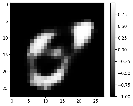
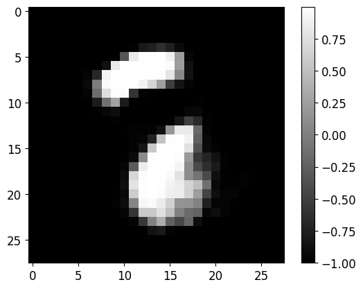
# 使用预先训练的解码器网络net_decoder将z样本解码为x样本
x_samples = net_decoder.decode(z_samples)
x_samples_np = x_samples if type(x_samples) is np.ndarray else x_samples.detach().numpy() # torch to numpy
for x_sample in x_samples_np:
plot_image(x_sample.reshape([H_height, W_width]))
# Lets finally run the synthesis and see what happens...
rng = np.random.RandomState(seed=SEED)
synthesize(net_decoder_pretrained,
rng,
min_z_wider, # From further above
max_z_wider, # From further above
n_samples=20)
5.8 使用 AE 从未标记数据中学习,以在标记数据有限时补充监督分类器:让我们首先“从头开始”训练一个监督分类器(Learning from Unlabelled data with AE, to complement Supervised Classifier when Labelled data are limited: Lets first train a supervised Classifier ‘from scratch’)
1
2
3
4
5
6
7
8
9
10
11
12
13
14
15
16
17
18
19
20
21
22
23
24
25
26
27
28
29
30
31
32
33
34
35
36
37
38
39
40
41
42
43
44
45
46
47
48
49
50
51
52
53
54
55
56
57
58
59
60
61
62
63
64
65
66
67
68
69
70
71
72
73
74
75
76
77
78
79
80
81
82
83
84
85
86
87
88
89
90
91
92
93
94
95
96
97
98
99
100
101
102
103
104
105
106
107
108
109
110
111
112
113
114
115
116
117
118
119
120
121
122
123
124
125
126
127
128
129
130
131
132
133
134
135
136
137
138
139
140
141
142
143
144
145
146
147
148
149
150
151
152
153
154
155
156
157
158
159
160
161
162
163
164
165
class Classifier_3layers(Network):
# 隐藏层使用ReLU激活函数,输出层使用softmax函数来计算类概率
def __init__(self, D_in, D_hid_1, D_hid_2, D_out, rng):
D_in = D_in
D_hid_1 = D_hid_1
D_hid_2 = D_hid_2
D_out = D_out
# === NOTE: Notice that this is exactly the same architecture as encoder of AE in Task 4 ====
w_1_init = rng.normal(loc=0.0, scale=0.01, size=(D_in+1, D_hid_1))
w_2_init = rng.normal(loc=0.0, scale=0.01, size=(D_hid_1+1, D_hid_2))
w_out_init = rng.normal(loc=0.0, scale=0.01, size=(D_hid_2+1, D_out))
w_1 = torch.tensor(w_1_init, dtype=torch.float, requires_grad=True)
w_2 = torch.tensor(w_2_init, dtype=torch.float, requires_grad=True)
w_out = torch.tensor(w_out_init, dtype=torch.float, requires_grad=True)
self.params = [w_1, w_2, w_out]
def forward_pass(self, batch_inp):
# compute predicted y
[w_1, w_2, w_out] = self.params
# In case input is image, make it a tensor.
batch_imgs_t = torch.tensor(batch_inp, dtype=torch.float) if type(batch_inp) is np.ndarray else batch_inp
unary_feature_for_bias = torch.ones(size=(batch_imgs_t.shape[0], 1)) # [N, 1] column vector.
x = torch.cat((batch_imgs_t, unary_feature_for_bias), dim=1) # Extra feature=1 for bias.
# === NOTE: This is the same architecture as encoder of AE in Task 4, with extra classification layer ===
# Layer 1
h1_preact = x.mm(w_1)
h1_act = h1_preact.clamp(min=0)
# Layer 2 (corresponds to bottleneck of the AE):
h1_ext = torch.cat((h1_act, unary_feature_for_bias), dim=1)
h2_preact = h1_ext.mm(w_2)
h2_act = h2_preact.clamp(min=0)
# Output classification layer
h2_ext = torch.cat((h2_act, unary_feature_for_bias), dim=1)
h_out = h2_ext.mm(w_out)
logits = h_out
# === Addition of a softmax function for
# Softmax activation function.
exp_logits = torch.exp(logits)
y_pred = exp_logits / torch.sum(exp_logits, dim=1, keepdim=True) # 使用softmax输出概率
# sum with Keepdim=True returns [N,1] array. It would be [N] if keepdim=False.
# Torch broadcasts [N,1] to [N,D_out] via repetition, to divide elementwise exp_h2 (which is [N,D_out]).
return y_pred
# 计算预测的类概率与真实类标签之间的交叉熵损失
# 在进行对数运算时,为了数值稳定性,添加了一个epsilon(eps)
def cross_entropy(y_pred, y_real, eps=1e-7):
# y_pred: Predicted class-posterior probabilities, returned by forward_pass. Numpy array of shape [N, D_out]
# y_real: One-hot representation of real training labels. Same shape as y_pred.
# If number array is given, change it to a Torch tensor.
y_pred = torch.tensor(y_pred, dtype=torch.float) if type(y_pred) is np.ndarray else y_pred
y_real = torch.tensor(y_real, dtype=torch.float) if type(y_real) is np.ndarray else y_real
x_entr_per_sample = - torch.sum( y_real*torch.log(y_pred+eps), dim=1) # Sum over classes, axis=1
loss = torch.mean(x_entr_per_sample, dim=0) # Expectation of loss: Mean over samples (axis=0).
return loss
from utils.plotting import plot_train_progress_2
def train_classifier(classifier,
pretrained_AE,
loss_func,
rng,
train_imgs,
train_lbls,
test_imgs,
test_lbls,
batch_size,
learning_rate,
total_iters,
iters_per_test=-1):
# Arguments:
# classifier: A classifier network. It will be trained by this function using labelled data.
# Its input will be either original data (if pretrained_AE=0), ...
# ... or the output of the feature extractor if one is given.
# pretrained_AE: A pretrained AutoEncoder that will *not* be trained here.
# It will be used to encode input data.
# The classifier will take as input the output of this feature extractor.
# If pretrained_AE = None: The classifier will simply receive the actual data as input.
# train_imgs: Vectorized training images
# train_lbls: One hot labels
# test_imgs: Vectorized testing images, to compute generalization accuracy.
# test_lbls: One hot labels for test data.
# batch_size: batch size
# learning_rate: come on...
# total_iters: how many SGD iterations to perform.
# iters_per_test: We will 'test' the model on test data every few iterations as specified by this.
values_to_plot = {'loss':[], 'acc_train': [], 'acc_test': []}
optimizer = optim.Adam(classifier.params, lr=learning_rate)
for t in range(total_iters):
# Sample batch for this SGD iteration
# 随机抽样一批数
train_imgs_batch, train_lbls_batch = get_random_batch(train_imgs, train_lbls, batch_size, rng)
# Forward pass执行前向传递以获得预测
if pretrained_AE is None:
inp_to_classifier = train_imgs_batch
else:
_, z_codes = pretrained_AE.forward_pass(train_imgs_batch) # AE encodes. Output will be given to Classifier
inp_to_classifier = z_codes
y_pred = classifier.forward_pass(inp_to_classifier)
# Compute loss:使用交叉熵函数计算损失
y_real = train_lbls_batch
loss = loss_func(y_pred, y_real) # Cross entropy
# Backprop and updates.使用反向传播计算梯度
optimizer.zero_grad()
grads = classifier.backward_pass(loss)
optimizer.step()
# ==== Report training loss and accuracy ======
# y_pred and loss can be either np.array, or torch.tensor (see later). If tensor, make it np.array.
y_pred_numpy = y_pred if type(y_pred) is np.ndarray else y_pred.detach().numpy()
y_pred_lbls = np.argmax(y_pred_numpy, axis=1) # y_pred is soft/probability. Make it a hard one-hot label.
y_real_lbls = np.argmax(y_real, axis=1)
acc_train = np.mean(y_pred_lbls == y_real_lbls) * 100. # percentage
loss_numpy = loss if type(loss) is type(float) else loss.item()
print("[iter:", t, "]: Training Loss: {0:.2f}".format(loss), "\t Accuracy: {0:.2f}".format(acc_train))
# =============== Every few iterations, show reconstructions ================#
if t==total_iters-1 or t%iters_per_test == 0:
if pretrained_AE is None:
inp_to_classifier_test = test_imgs
else:
_, z_codes_test = pretrained_AE.forward_pass(test_imgs)
inp_to_classifier_test = z_codes_test
y_pred_test = classifier.forward_pass(inp_to_classifier_test)
# ==== Report test accuracy ======
y_pred_test_numpy = y_pred_test if type(y_pred_test) is np.ndarray else y_pred_test.detach().numpy()
y_pred_lbls_test = np.argmax(y_pred_test_numpy, axis=1)
y_real_lbls_test = np.argmax(test_lbls, axis=1)
acc_test = np.mean(y_pred_lbls_test == y_real_lbls_test) * 100.
print("\t\t\t\t\t\t\t\t Testing Accuracy: {0:.2f}".format(acc_test))
# Keep list of metrics to plot progress.
values_to_plot['loss'].append(loss_numpy)
values_to_plot['acc_train'].append(acc_train)
values_to_plot['acc_test'].append(acc_test)
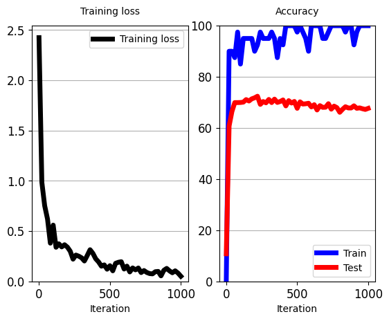
# In the end of the process, plot loss accuracy on training and testing data.
plot_train_progress_2(values_to_plot['loss'], values_to_plot['acc_train'], values_to_plot['acc_test'], iters_per_test)
1
2
3
4
5
6
7
8
9
10
11
12
13
14
15
16
17
18
19
20
21
22
23
24
25
26
27
28
29
30
31
32
33
34
35
36
37
38
# Train Classifier from scratch (initialized randomly)

# Create the network
rng = np.random.RandomState(seed=SEED)
net_classifier_from_scratch = Classifier_3layers(D_in=H_height*W_width,
                                                 D_hid_1=256, # TODO: Use same as layer 1 of encoder of wide AE (Task 4)
                                                 D_hid_2=32,  # TODO: Use same as layer 1 of encoder of wide AE (Task 4)
                                                 D_out=C_classes,
                                                 rng=rng)
# Start training
train_classifier(net_classifier_from_scratch,
                 None,  # No pretrained AE
                 cross_entropy,
                 rng,
                 train_imgs_flat[:100],
                 train_lbls_onehot[:100],
                 test_imgs_flat,
                 test_lbls_onehot,
                 batch_size=40,
                 learning_rate=3e-3,
                 total_iters=1000,
                 iters_per_test=20)

'''
[iter: 16 ]: Training Loss: 1.93 	 Accuracy: 32.50
[iter: 17 ]: Training Loss: 2.04 	 Accuracy: 30.00
[iter: 18 ]: Training Loss: 1.91 	 Accuracy: 27.50
[iter: 19 ]: Training Loss: 1.77 	 Accuracy: 32.50
[iter: 20 ]: Training Loss: 1.71 	 Accuracy: 40.00
								 Testing Accuracy: 30.05
[iter: 21 ]: Training Loss: 1.67 	 Accuracy: 42.50
[iter: 22 ]: Training Loss: 1.64 	 Accuracy: 57.50
...
[iter: 997 ]: Training Loss: 0.00 	 Accuracy: 100.00
[iter: 998 ]: Training Loss: 0.00 	 Accuracy: 100.00
[iter: 999 ]: Training Loss: 0.00 	 Accuracy: 100.00
								 Testing Accuracy: 55.60
'''

5.9 当标签有限时,使用无监督 AE 作为监督分类器的“预训练特征提取器”(Use Unsupervised AE as ‘pre-trained feature-extractor’ for a supervised Classifier when labels are limited)
1
2
3
4
5
6
7
8
9
10
11
12
13
14
15
16
17
18
19
20
21
22
23
24
25
26
27
28
29
30
31
32
33
34
35
36
37
38
39
40
41
42
43
44
45
46
47
48
49
50
51
52
53
54
55
56
57
58
59
60
61
62
63
64
65
66
67
68
69
70
71
72
73
74
75
76
77
78
79
80
81
82
83
84
85
86
87
88
89
90
91
92
93
94
# Train classifier on top of pre-trained AE encoder

class Classifier_1layer(Network):
    # Classifier with just 1 layer, the classification layer
    def __init__(self, D_in, D_out, rng):
        # D_in: dimensions of input
        # D_out: dimension of output (number of classes)

        #### TODO: Fill in the blanks ######################
        w_out_init = rng.normal(loc=0.0, scale=0.01, size=(D_in+1, D_out))
        w_out = torch.tensor(w_out_init, dtype=torch.float, requires_grad=True)
        ####################################################
        self.params = [w_out]


    def forward_pass(self, batch_inp):
        # compute predicted y
        [w_out] = self.params

        # In case input is image, make it a tensor.
        batch_inp_t = torch.tensor(batch_inp, dtype=torch.float) if type(batch_inp) is np.ndarray else batch_inp

        unary_feature_for_bias = torch.ones(size=(batch_inp_t.shape[0], 1)) # [N, 1] column vector.
        batch_inp_ext = torch.cat((batch_inp_t, unary_feature_for_bias), dim=1) # Extra feature=1 for bias. Lec5, slide 4.

        # Output classification layer
        logits = batch_inp_ext.mm(w_out)

        # Output layer activation function
        # Softmax activation function. See Lecture 5, slide 18.
        exp_logits = torch.exp(logits)
        y_pred = exp_logits / torch.sum(exp_logits, dim=1, keepdim=True)
        # sum with Keepdim=True returns [N,1] array. It would be [N] if keepdim=False.
        # Torch broadcasts [N,1] to [N,D_out] via repetition, to divide elementwise exp_h2 (which is [N,D_out]).

        return y_pred


# Create the network
rng = np.random.RandomState(seed=SEED) # Random number generator
# As input, it will be getting z-codes from the AE with 32-neurons bottleneck from Task 4.
classifier_1layer = Classifier_1layer(autoencoder_wide.D_bottleneck,  # Input dimension is dimensions of AE's Z
                                      C_classes,
                                      rng=rng)

########### TODO: Fill in the gaps to start training ####################
# Give to the function the 1-layer classifier, as well as the pre-trained AE that will work as feature extractor.
# For the pre-trained AE, give the instance of 'wide' AE that has 32-neurons bottleneck, which you trained in Task 4.
train_classifier(classifier_1layer,  # 要训练的单层分类器
                 autoencoder_wide,  # 预训练的AE,将被用作特征提取器
                 cross_entropy,  # 计算损失的函数
                 rng,
                 train_imgs_flat[:100],
                 train_lbls_onehot[:100],
                 test_imgs_flat,
                 test_lbls_onehot,
                 batch_size=40,
                 learning_rate=3e-3,   # 5e-3, is the best for 1-layer classifier and all data.
                 total_iters=1000,
                 iters_per_test=20)

'''
[iter: 0 ]: Training Loss: 2.42 	 Accuracy: 0.00
								 Testing Accuracy: 10.79
[iter: 1 ]: Training Loss: 2.25 	 Accuracy: 12.50
[iter: 2 ]: Training Loss: 2.08 	 Accuracy: 20.00
[iter: 3 ]: Training Loss: 2.16 	 Accuracy: 7.50
[iter: 4 ]: Training Loss: 1.99 	 Accuracy: 35.00
[iter: 5 ]: Training Loss: 1.78 	 Accuracy: 60.00
[iter: 6 ]: Training Loss: 1.90 	 Accuracy: 32.50
[iter: 7 ]: Training Loss: 1.79 	 Accuracy: 47.50
[iter: 8 ]: Training Loss: 1.74 	 Accuracy: 45.00
[iter: 9 ]: Training Loss: 1.67 	 Accuracy: 50.00
[iter: 10 ]: Training Loss: 1.57 	 Accuracy: 62.50
[iter: 11 ]: Training Loss: 1.51 	 Accuracy: 67.50
[iter: 12 ]: Training Loss: 1.37 	 Accuracy: 72.50
[iter: 13 ]: Training Loss: 1.43 	 Accuracy: 77.50
[iter: 14 ]: Training Loss: 1.37 	 Accuracy: 65.00
[iter: 15 ]: Training Loss: 1.33 	 Accuracy: 60.00
[iter: 16 ]: Training Loss: 1.44 	 Accuracy: 65.00
[iter: 17 ]: Training Loss: 1.41 	 Accuracy: 72.50
[iter: 18 ]: Training Loss: 1.39 	 Accuracy: 70.00
[iter: 19 ]: Training Loss: 1.17 	 Accuracy: 72.50
[iter: 20 ]: Training Loss: 0.99 	 Accuracy: 90.00
								 Testing Accuracy: 60.76
[iter: 21 ]: Training Loss: 1.09 	 Accuracy: 87.50
[iter: 22 ]: Training Loss: 1.01 	 Accuracy: 80.00
...
[iter: 997 ]: Training Loss: 0.04 	 Accuracy: 100.00
[iter: 998 ]: Training Loss: 0.09 	 Accuracy: 100.00
[iter: 999 ]: Training Loss: 0.05 	 Accuracy: 100.00
								 Testing Accuracy: 67.65
'''
5.10 使用无监督 AE 编码器的参数来初始化监督分类器的权重,然后使用有限的标签进行细化(Use parameters of an Unsupervised AE’s encoder to initialize weights of a supervised Classifier, followed by refinement using limited labels)
1
2
3
4
5
6
7
8
9
10
11
12
13
14
15
16
17
18
19
20
21
22
23
24
25
26
27
28
29
30
31
32
33
34
35
36
37
38
39
40
41
42
43
44
45
46
47
48
49
50
51
52
53
54
55
56
57
58
59
60
61
62
63
64
65
66
67
68
69
70
71
72
73
74
75
76
77
78
79
# Pre-train a classifier.

# The below classifier has THE SAME architecture as the 3-layer Classifier that we trained...
# ... in a purely supervised manner in Task-6.
# This is done by inheriting the class (Classifier_3layers), therefore uses THE SAME forward_pass() function.
# THE ONLY DIFFERENCE is in the construction __init__.
# This 'pretrained' classifier receives as input a pretrained autoencoder (pretrained_AE) from Task 4.
# It then uses the parameters of the AE's encoder to initialize its own parameters, rather than random initialization.
# The model is then trained all together.
class Classifier_3layers_pretrained(Classifier_3layers):
    def __init__(self, pretrained_AE, D_in, D_out, rng):
        D_in = D_in
        D_hid_1 = 256
        D_hid_2 = 32
        D_out = D_out

        w_out_init = rng.normal(loc=0.0, scale=0.01, size=(D_hid_2+1, D_out))

        w_1 = torch.tensor(pretrained_AE.params[0], dtype=torch.float, requires_grad=True)
        w_2 = torch.tensor(pretrained_AE.params[1], dtype=torch.float, requires_grad=True)
        w_out = torch.tensor(w_out_init, dtype=torch.float, requires_grad=True)

        self.params = [w_1, w_2, w_out]

# Create the network
rng = np.random.RandomState(seed=SEED) # Random number generator
classifier_3layers_pretrained = Classifier_3layers_pretrained(autoencoder_wide,  # The AE pre-trained in Task 4.
                                                              train_imgs_flat.shape[1],
                                                              C_classes,
                                                              rng=rng)

# Start training
# NOTE: Only the 3-layer pretrained classifier is used, and will be trained all together.
# No frozen feature extractor.
train_classifier(classifier_3layers_pretrained,  # classifier that will be trained.
                 None,  # No pretrained AE to act as 'frozen' feature extractor.
                 cross_entropy,
                 rng,
                 train_imgs_flat[:100],
                 train_lbls_onehot[:100],
                 test_imgs_flat,
                 test_lbls_onehot,
                 batch_size=40,
                 learning_rate=3e-3,
                 total_iters=1000,
                 iters_per_test=20)

'''
[iter: 0 ]: Training Loss: 2.42 	 Accuracy: 0.00
								 Testing Accuracy: 12.06
[iter: 1 ]: Training Loss: 2.19 	 Accuracy: 12.50
[iter: 2 ]: Training Loss: 2.04 	 Accuracy: 22.50
[iter: 3 ]: Training Loss: 2.11 	 Accuracy: 15.00
[iter: 4 ]: Training Loss: 1.89 	 Accuracy: 50.00
[iter: 5 ]: Training Loss: 1.68 	 Accuracy: 67.50
[iter: 6 ]: Training Loss: 1.71 	 Accuracy: 42.50
[iter: 7 ]: Training Loss: 1.58 	 Accuracy: 57.50
[iter: 8 ]: Training Loss: 1.55 	 Accuracy: 60.00
[iter: 9 ]: Training Loss: 1.36 	 Accuracy: 65.00
[iter: 10 ]: Training Loss: 1.18 	 Accuracy: 65.00
[iter: 11 ]: Training Loss: 1.12 	 Accuracy: 67.50
[iter: 12 ]: Training Loss: 0.88 	 Accuracy: 70.00
[iter: 13 ]: Training Loss: 0.98 	 Accuracy: 62.50
[iter: 14 ]: Training Loss: 0.86 	 Accuracy: 75.00
[iter: 15 ]: Training Loss: 0.72 	 Accuracy: 80.00
[iter: 16 ]: Training Loss: 0.93 	 Accuracy: 77.50
[iter: 17 ]: Training Loss: 0.84 	 Accuracy: 82.50
[iter: 18 ]: Training Loss: 0.78 	 Accuracy: 80.00
[iter: 19 ]: Training Loss: 0.44 	 Accuracy: 92.50
[iter: 20 ]: Training Loss: 0.55 	 Accuracy: 87.50
								 Testing Accuracy: 62.03
[iter: 21 ]: Training Loss: 0.46 	 Accuracy: 87.50
[iter: 22 ]: Training Loss: 0.48 	 Accuracy: 90.00
...
[iter: 997 ]: Training Loss: 0.00 	 Accuracy: 100.00
[iter: 998 ]: Training Loss: 0.00 	 Accuracy: 100.00
[iter: 999 ]: Training Loss: 0.00 	 Accuracy: 100.00
								 Testing Accuracy: 69.20
'''
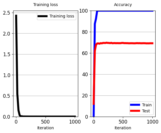
与Classifier_1layer相比,Classifier_3layers_pretrained有以下主要区别:
- 层数和复杂性:
Classifier_1layer只有一个输出层。它直接从输入层转到输出层,因此只有一个层。Classifier_3layers_pretrained有三层:两个隐藏层和一个输出层。这增加了网络的复杂性。
- 参数初始化:
Classifier_1layer使用随机初始化来设置其权重。Classifier_3layers_pretrained使用预训练的自动编码器(AE)的前两层的权重来初始化其前两层的权重。输出层的权重仍然是随机初始化的。
- 参数数量:
Classifier_1layer只有一层的权重。Classifier_3layers_pretrained有三层的权重,因此它有更多的参数,需要更多的计算和存储。
- 继承:
Classifier_1layer是一个独立的网络类。Classifier_3layers_pretrained继承自Classifier_3layers,这意味着它重用了Classifier_3layers的某些方法,特别是forward_pass()方法。它们的主要区别是在初始化函数__init__中。
- 用途:
Classifier_1layer主要用于在预训练的AE编码器上进行分类,AE编码器用作特征提取器。Classifier_3layers_pretrained是完全训练的,即使它使用了预训练的AE的权重来初始化,但在训练过程中,所有的权重都会更新。
6. 变分自动编码器 (VAE) Variational Auto-Encoders(VAEs)
6.1 加载并刷新 MNIST Loading and Refresshing MNIST
1
2
3
4
5
6
7
8
9
10
11
12
13
14
15
16
17
18
19
20
21
22
23
24
25
26
27
28
29
# -*- coding: utf-8 -*-
# The below is for auto-reloading external modules after they are changed, such as those in ./utils.
# Issue: https://stackoverflow.com/questions/1907993/autoreload-of-modules-in-ipython
%load_ext autoreload
%autoreload 2

import numpy as np
from utils.data_utils import get_mnist # Helper function. Use it out of the box.

# Constants
DATA_DIR = './data/mnist' # Location we will keep the data.
SEED = 111111

# If datasets are not at specified location, they will be downloaded.
train_imgs, train_lbls = get_mnist(data_dir=DATA_DIR, train=True, download=True)
test_imgs, test_lbls = get_mnist(data_dir=DATA_DIR, train=False, download=True)

print("[train_imgs] Type: ", type(train_imgs), "|| Shape:", train_imgs.shape, "|| Data type: ", train_imgs.dtype )
print("[train_lbls] Type: ", type(train_lbls), "|| Shape:", train_lbls.shape, "|| Data type: ", train_lbls.dtype )
print('Class labels in train = ', np.unique(train_lbls))

print("[test_imgs] Type: ", type(test_imgs), "|| Shape:", test_imgs.shape, " || Data type: ", test_imgs.dtype )
print("[test_lbls] Type: ", type(test_lbls), "|| Shape:", test_lbls.shape, " || Data type: ", test_lbls.dtype )
print('Class labels in test = ', np.unique(test_lbls))

N_tr_imgs = train_imgs.shape[0] # N hereafter. Number of training images in database.
H_height = train_imgs.shape[1] # H hereafter
W_width = train_imgs.shape[2] # W hereafter
C_classes = len(np.unique(train_lbls)) # C hereafter
1
2
3
%matplotlib inline
from utils.plotting import plot_grid_of_images # Helper functions, use out of the box.
plot_grid_of_images(train_imgs[0:100], n_imgs_per_row=10)
6.2 数据预处理 Data pre-processing
1
2
3
4
5
6
7
# a) Change representation of labels to one-hot vectors of length C=10.
train_lbls_onehot = np.zeros(shape=(train_lbls.shape[0], C_classes ) )
train_lbls_onehot[ np.arange(train_lbls_onehot.shape[0]), train_lbls ] = 1
test_lbls_onehot = np.zeros(shape=(test_lbls.shape[0], C_classes ) )
test_lbls_onehot[ np.arange(test_lbls_onehot.shape[0]), test_lbls ] = 1
print("BEFORE: [train_lbls]        Type: ", type(train_lbls), "|| Shape:", train_lbls.shape, " || Data type: ", train_lbls.dtype )
print("AFTER : [train_lbls_onehot] Type: ", type(train_lbls_onehot), "|| Shape:", train_lbls_onehot.shape, " || Data type: ", train_lbls_onehot.dtype )
1
2
3
4
5
6
7
8
9
10
11
12
13
14
15
16
# b) Re-scale image intensities, from [0,255] to [-1, +1].
# This commonly facilitates learning:
# A zero-centered signal with small magnitude allows avoiding exploding/vanishing problems easier.
from utils.data_utils import normalize_int_whole_database # Helper function. Use out of the box.
train_imgs = normalize_int_whole_database(train_imgs, norm_type="minus_1_to_1")
test_imgs = normalize_int_whole_database(test_imgs, norm_type="minus_1_to_1")

# Lets plot one image.
from utils.plotting import plot_image, plot_images # Helper function, use out of the box.
index = 0  # Try any, up to 60000
print("Plotting image of index: [", index, "]")
print("Class label for this image is: ", train_lbls[index])
print("One-hot label representation: [", train_lbls_onehot[index], "]")
plot_image(train_imgs[index])
# Notice the magnitude of intensities. Black is now negative and white is positive float.
# Compare with intensities of figure further above.
1
2
3
4
5
6
# c) Flatten the images, from 2D matrices to 1D vectors. MLPs take feature-vectors as input, not 2D images.
train_imgs_flat = train_imgs.reshape([train_imgs.shape[0], -1]) # Preserve 1st dim (S = num Samples), flatten others.
test_imgs_flat = test_imgs.reshape([test_imgs.shape[0], -1])
print("Shape of numpy array holding the training database:")
print("Original : [N, H, W] = [", train_imgs.shape , "]")
print("Flattened: [N, H*W]  = [", train_imgs_flat.shape , "]")
6.3 变分自动编码器 Variational Auto-Encoder
1
2
3
4
5
6
7
8
9
10
11
12
13
14
15
16
17
18
19
20
21
22
23
24
25
26
27
28
29
30
31
32
33
34
35
36
37
38
39
40
41
42
43
44
45
46
47
48
49
50
51
52
53
54
55
56
57
58
59
60
61
62
63
64
65
66
67
68
69
70
71
72
73
74
75
76
77
78
79
80
81
82
83
84
85
86
87
88
89
90
91
92
93
94
95
96
97
98
99
100
101
102
103
104
105
106
107
108
109
110
111
112
113
114
115
116
117
118
119
120
121
122
123
124
125
126
127
128
129
130
131
132
133
134
135
136
137
138
139
140
141
142
143
144
145
146
147
148
149
150
151
152
153
154
155
156
157
158
159
160
161
162
163
164
165
166
167
168
169
170
171
172
173
174
175
176
177
178
179
180
import torch
import torch.optim as optim
import torch.nn as nn

class Network():
    def backward_pass(self, loss):
        # Performs back propagation and computes gradients
        # With PyTorch, we do not need to compute gradients analytically for parameters were requires_grads=True,
        # Calling loss.backward(), torch's Autograd automatically computes grads of loss wrt each parameter p,...
        # ... and **puts them in p.grad**. Return them in a list.
        loss.backward()
        grads = [param.grad for param in self.params]
        return grads

class VAE(Network):
    def __init__(self, rng, D_in, D_hid_enc, D_bottleneck, D_hid_dec):
        # Construct and initialize network parameters
        D_in = D_in # Dimension of input feature-vectors. Length of a vectorised image.
        D_hid_1 = D_hid_enc # Dimension of Encoder's hidden layer
        D_hid_2 = D_bottleneck
        D_hid_3 = D_hid_dec  # Dimension of Decoder's hidden layer
        D_out = D_in # Dimension of Output layer.

        self.D_bottleneck = D_bottleneck  # Keep track of it, we will need it.

        ##### TODO: Initialize the VAE's parameters. Also see forward_pass(...)) ########
        # Dimensions of parameter tensors are (number of neurons + 1) per layer, to account for +1 bias.
        # -- (Encoder) layer 1
        w1_init = rng.normal(loc=0.0, scale=0.01, size=(D_in+1, D_hid_1))
        # -- (Encoder) layer 2, predicting p(z|x)
        w2_mu_init = rng.normal(loc=0.0, scale=0.01, size=(D_hid_1+1, D_hid_2))
        w2_std_init = rng.normal(loc=0.0, scale=0.01, size=(D_hid_1+1, D_hid_2))
        # -- (Decoder) layer 3
        w3_init = rng.normal(loc=0.0, scale=0.01, size=(D_hid_2+1, D_hid_3))
        # -- (Decoder) layer 4, the output layer
        w4_init = rng.normal(loc=0.0, scale=0.01, size=(D_hid_3+1, D_out))

        # Pytorch tensors, parameters of the model
        # Use the above numpy arrays as of random floats as initialization for the Pytorch weights.
        # (Encoder)
        w1 = torch.tensor(w1_init, dtype=torch.float, requires_grad=True)
        # (Encoder) Layer 2, predicting p(z|x)
        w2_mu = torch.tensor(w2_mu_init, dtype=torch.float, requires_grad=True)
        w2_std = torch.tensor(w2_std_init, dtype=torch.float, requires_grad=True)
        # (Decoder)
        w3 = torch.tensor(w3_init, dtype=torch.float, requires_grad=True)
        w4 = torch.tensor(w4_init, dtype=torch.float, requires_grad=True)
        # Keep track of all trainable parameters:
        self.params = [w1, w2_mu, w2_std, w3, w4]
        ###########################################################################


    def encode(self, batch_imgs):
        # batch_imgs: Numpy array or Pytorch tensor of shape: [number of inputs, dimensionality of x]
        [w1, w2_mu, w2_std, w3, w4] = self.params

        batch_imgs_t = torch.tensor(batch_imgs, dtype=torch.float) if type(batch_imgs) is np.ndarray else batch_imgs

        unary_feature_for_bias = torch.ones(size=(batch_imgs_t.shape[0], 1)) # [N, 1] column vector.
        x = torch.cat((batch_imgs_t, unary_feature_for_bias), dim=1) # Extra feature=1 for bias.

        # ========== TODO: Fill in the gaps with the correct parameters of the VAE ========
        # Encoder's Layer 1
        h1_preact = x.mm(w1)
        h1_act = h1_preact.clamp(min=0)
        # Encoder's Layer 2 (predicting p(z|x) of Z coding):
        h1_ext = torch.cat((h1_act, unary_feature_for_bias), dim=1)
        # ... mu
        h2_mu_preact = h1_ext.mm(w2_mu)   # <------------- ????????
        h2_mu_act = h2_mu_preact
        # ... log(std). Ask yourselves: Why do we do this, instead of directly predicting std deviation?
        h2_logstd_preact = h1_ext.mm(w2_std)  # <-------------- ???????
        h2_logstd_act = h2_logstd_preact  # No (linear) activation function in this tutorial, but can use any.
        # ==============================================================================

        z_coding = (h2_mu_act, h2_logstd_act)

        return z_coding


    def decode(self, z_codes):
        # z_codes: numpy array or pytorch tensor, shape [N, dimensionality of Z]
        [w1, w2_mu, w2_std, w3, w4] = self.params

        z_codes_t = torch.tensor(z_codes, dtype=torch.float) if type(z_codes) is np.ndarray else z_codes

        unary_feature_for_bias = torch.ones(size=(z_codes_t.shape[0], 1)) # [N, 1] column vector.

        # ========== TODO: Fill in the gaps with the correct parameters of the VAE ========
        # Decoder's 1st layer (Layer 3 of whole VAE):
        h2_ext = torch.cat((z_codes_t, unary_feature_for_bias), dim=1)
        h3_preact = h2_ext.mm(w3)  # < ----------------------------------
        h3_act = h3_preact.clamp(min=0)
        # Decoder's 2nd layer (Layer 4 of whole VAE): The output layer.
        h3_ext = torch.cat((h3_act, unary_feature_for_bias), dim=1)
        h4_preact = h3_ext.mm(w4)
        h4_act = torch.tanh(h4_preact)
        # ==============================================================================

        # Output
        x_pred = h4_act

        return x_pred


    def sample_with_reparameterization(self, z_mu, z_logstd):
        # Reparameterization trick to sample from N(mu, var) using N(0,1) as intermediate step.
        # param z_mu: Tensor. Mean of the predicted Gaussian p(z|x). Shape: [Num samples, Dimensionality of Z]
        # param z_logstd: Tensor. Log of standard deviation of predicted Gaussian p(z|x). [Num samples, Dim of Z]
        # return: Tensor. [Num samples, Dim of Z]

        N_samples = z_mu.shape[0]
        Z_dims = z_mu.shape[1]

        # ========== TODO: Fill in the gaps to complete the reparameterization trick ========
        z_std = torch.exp(z_logstd)       #   <--------------- ?????????
        eps = torch.randn(size=[N_samples, Z_dims])  # Samples from N(0,I)
        z_samples = z_mu + z_std * eps    #           <--------------- ?????????
        # ==============================================================================

        return z_samples


    def forward_pass(self, batch_imgs):
        batch_imgs_t = torch.tensor(batch_imgs, dtype=torch.float)  # Makes numpy array to pytorch tensor.

        # ========== TODO: Call the appropriate functions, as you defined them above ========
        # Encoder
        z_mu, z_logstd = self.encode(batch_imgs_t)  # <------------- ????????????
        z_samples = self.sample_with_reparameterization(z_mu, z_logstd)  # <------------- ????????????
        # Decoder
        x_pred = self.decode(z_samples)  # <------------- ????????????
        # ===================================================================================

        return (x_pred, z_mu, z_logstd, z_samples)

def reconstruction_loss(x_pred, x_real, eps=1e-7):
    # x_pred: [N, D_out] Prediction returned by forward_pass. Numpy array of shape [N, D_out]
    # x_real: [N, D_in]

    # If number array is given, change it to a Torch tensor.
    x_pred = torch.tensor(x_pred, dtype=torch.float) if type(x_pred) is np.ndarray else x_pred
    x_real = torch.tensor(x_real, dtype=torch.float) if type(x_real) is np.ndarray else x_real

    ######## TODO: Complete the calculation of Reconstruction loss for each sample ###########
    loss_recon = torch.mean(torch.square(x_pred - x_real), dim=1)
    ##########################################################################################

    cost = torch.mean(loss_recon, dim=0) # Expectation of loss: Mean over samples (axis=0).

    return cost


def regularizer_loss(mu, log_std):
    # mu: Tensor, [number of samples, dimensionality of Z]. Predicted means per z dimension
    # log_std: Tensor, [number of samples, dimensionality of Z]. Predicted log(std.dev.) per z dimension.

    ######## TODO: Complete the calculation of Reconstruction loss for each sample ###########
    std = torch.exp(log_std)  # Compute std.dev. from log(std.dev.)
    reg_loss_per_sample = 0.5 * torch.sum(mu**2 + std**2 - 2 * log_std - 1, dim = 1)  # <----------
    reg_loss = torch.mean(reg_loss_per_sample, dim = 0)  # Mean over samples.
    ##########################################################################################

    return reg_loss


def vae_loss(x_real, x_pred, z_mu, z_logstd, lambda_rec=1., lambda_reg=0.005, eps=1e-7):

    rec_loss = reconstruction_loss(x_pred, x_real, eps=1e-7)
    reg_loss = regularizer_loss(z_mu, z_logstd)

    ################### TODO: compute the total loss: #####################################
    # ...by weighting the reconstruction loss by lambda_rec, and the Regularizer by lambda_reg
    weighted_rec_loss = lambda_rec * rec_loss
    weighted_reg_loss = lambda_reg * reg_loss
    total_loss = weighted_rec_loss + weighted_reg_loss
    #######################################################################################

    return total_loss, weighted_rec_loss, weighted_reg_loss
6.4 VAE的无监督训练 Unsupervised training of VAE
1
2
3
4
5
6
7
8
9
10
11
12
13
14
15
16
17
18
19
20
21
22
23
24
25
26
27
28
29
30
31
32
33
34
35
36
37
38
39
40
41
42
43
44
45
46
47
48
49
50
51
52
53
54
55
56
57
58
59
60
61
62
63
64
65
66
67
68
69
70
71
72
73
74
75
76
77
78
79
80
81
82
83
84
85
86
87
88
89
90
91
92
93
94
from utils.plotting import plot_train_progress_VAE, plot_grids_of_images  # Use out of the box


def get_random_batch(train_imgs, train_lbls, batch_size, rng):
    # train_imgs: Images. Numpy array of shape [N, H * W]
    # train_lbls: Labels of images. None, or Numpy array of shape [N, C_classes], one hot label for each image.
    # batch_size: integer. Size that the batch should have.

    indices = range(0, batch_size)  # Remove this line after you fill-in and un-comment the below.
    indices = rng.randint(low=0, high=train_imgs.shape[0], size=batch_size, dtype='int32')

    train_imgs_batch = train_imgs[indices]
    if train_lbls is not None:  # Enables function to be used both for supervised and unsupervised learning
        train_lbls_batch = train_lbls[indices]
    else:
        train_lbls_batch = None
    return [train_imgs_batch, train_lbls_batch]


def unsupervised_training_VAE(net,
                             loss_func,
                             lambda_rec,
                             lambda_reg,
                             rng,
                             train_imgs_all,
                             batch_size,
                             learning_rate,
                             total_iters,
                             iters_per_recon_plot=-1):
    # net: Instance of a model. See classes: Autoencoder, MLPClassifier, etc further below
    # loss_func: Function that computes the loss. See functions: reconstruction_loss or cross_entropy.
    # lambda_rec: weighing of reconstruction loss in total loss. Total = lambda_rec * rec_loss + lambda_reg * reg_loss
    # lambda_reg: same as above, but for regularizer
    # rng: numpy random number generator
    # train_imgs_all: All the training images. Numpy array, shape [N_tr, H, W]
    # batch_size: Size of the batch that should be processed per SGD iteration by a model.
    # learning_rate: self explanatory.
    # total_iters: how many SGD iterations to perform.
    # iters_per_recon_plot: Integer. Every that many iterations the model predicts training images ...
    #                      ...and we plot their reconstruction. For visual observation of the results.
    loss_total_to_plot = []
    loss_rec_to_plot = []
    loss_reg_to_plot = []

    optimizer = optim.Adam(net.params, lr=learning_rate)  # Will use PyTorch's Adam optimizer out of the box

    for t in range(total_iters):
        # Sample batch for this SGD iteration
        x_batch, _ = get_random_batch(train_imgs_all, None, batch_size, rng)

        ################### TODO: compute the total loss: ################################################
        # Pass parameters of the predicted distribution per x (mean mu and log(std.dev) to the loss function

        # Forward pass: Encodes, samples via reparameterization trick, decodes
        x_pred, z_mu, z_logstd, z_codes = net.forward_pass(x_batch)

        # Compute loss:
        total_loss, rec_loss, reg_loss = loss_func(x_batch, x_pred, z_mu, z_logstd, lambda_rec, lambda_reg) # <-------------
        ####################################################################################################
        # Pytorch way
        optimizer.zero_grad()
        _ = net.backward_pass(total_loss)
        optimizer.step()

        # ==== Report training loss and accuracy ======
        total_loss_np = total_loss if type(total_loss) is type(float) else total_loss.item()  # Pytorch returns tensor. Cast to float
        rec_loss_np = rec_loss if type(rec_loss) is type(float) else rec_loss.item()
        reg_loss_np = reg_loss if type(reg_loss) is type(float) else reg_loss.item()
        if t%10==0:  # Print every 10 iterations
            print("[iter:", t, "]: Total training Loss: {0:.2f}".format(total_loss_np))
        loss_total_to_plot.append(total_loss_np)
        loss_rec_to_plot.append(rec_loss_np)
        loss_reg_to_plot.append(reg_loss_np)

        # =============== Every few iterations, show reconstructions ================#
        if t==total_iters-1 or t%iters_per_recon_plot == 0:
            # Reconstruct all images, to plot reconstructions.
            x_pred_all, z_mu_all, z_logstd_all, z_codes_all = net.forward_pass(train_imgs_all)
            # Cast tensors to numpy arrays
            x_pred_all_np = x_pred_all if type(x_pred_all) is np.ndarray else x_pred_all.detach().numpy()

            # Predicted reconstructions have vector shape. Reshape them to original image shape.
            train_imgs_resh = train_imgs_all.reshape([train_imgs_all.shape[0], H_height, W_width])
            x_pred_all_np_resh = x_pred_all_np.reshape([train_imgs_all.shape[0], H_height, W_width])

            # Plot a few images, originals and predicted reconstructions.
            plot_grids_of_images([train_imgs_resh[0:100], x_pred_all_np_resh[0:100]],
                                  titles=["Real", "Reconstructions"],
                                  n_imgs_per_row=10,
                                  dynamically=True)

    # In the end of the process, plot loss.
    plot_train_progress_VAE(loss_total_to_plot, loss_rec_to_plot, loss_reg_to_plot, iters_per_point=1, y_lims=[1., 1., None])
1
2
3
4
5
6
7
8
9
10
11
12
13
14
15
16
17
18
19
20
21
##################### TODO: Fill in the blank ##############################
# Create the network
rng = np.random.RandomState(seed=SEED)
vae = VAE(rng=rng,
          D_in=H_height*W_width,
          D_hid_enc=256,
          D_bottleneck=2,  # <--- Set to correct value for instantiating VAE shown & implemented in Task 1. Note: We treat D as dimensionality of Z, rather than number of neurons.
          D_hid_dec=256)
########################################################################
# Start training
unsupervised_training_VAE(vae,
                          vae_loss,
                          lambda_rec=1.0,  # <-------- lambda_rec, weight on reconstruction loss.
                          lambda_reg=0.005,  # <------- lambda_reg, weight on regularizer. 0.005 works ok.
                          rng=rng,
                          train_imgs_all=train_imgs_flat,
                          batch_size=40,
                          learning_rate=3e-3,
                          total_iters=1000,
                          iters_per_recon_plot=50)
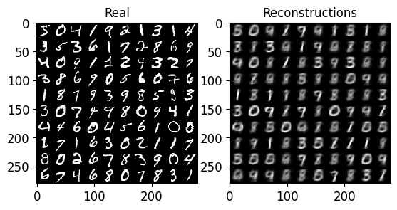
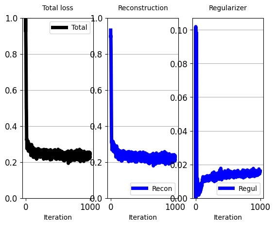
6.5 以 Z 表示形式对训练数据进行编码并检查 Encode training data in Z representation and examine
1
2
3
4
5
6
7
8
9
10
11
12
13
14
15
16
17
18
19
20
21
22
23
24
25
26
27
28
29
30
31
32
33
34
35
36
37
38
39
40
41
42
43
44
45
46
47
48
49
50
51
52
53
54
55
56
57
58
59
60
61
62
63
64
65
66
67
68
69
70
71
72
73
74
import matplotlib.pyplot as plt

def encode_training_images(net,
                           imgs_flat,
                           lbls,
                           batch_size,
                           total_iterations=None,
                           plot_2d_embedding=True,
                           plot_hist_mu_std_for_dim=0):
    # This function encodes images, plots the first 2 dimensions of the codes in a plot, and finally...
    # ... returns the minimum and maximum values of the codes for each dimensions of Z.
    # ... We will use  this at a layer task.
    # Arguments:
    # imgs_flat: Numpy array of shape [Number of images, H * W]
    # lbls: Numpy array of shape [number of images], with 1 integer per image. The integer is the class (digit).
    # total_iterations: How many batches to encode. We will use this so that we dont encode and plot ...
    # ... the whoooole training database, because the plot will get cluttered with 60000 points.
    # Returns:
    # min_z: numpy array, vector with [dimensions-of-z] elements. Minimum value per dimension of z.
    # max_z: numpy array, vector with [dimensions-of-z] elements. Maximum value per dimension of z.

    # If total iterations is None, the function will just iterate over all data, by breaking them into batches.
    if total_iterations is None:
        total_iterations = (train_imgs_flat.shape[0] - 1) // batch_size + 1

    z_mu_all = []
    z_std_all = []
    lbls_all = []
    for t in range(total_iterations):
        # Sample batch for this SGD iteration
        x_batch = imgs_flat[t*batch_size: (t+1)*batch_size]
        lbls_batch = lbls[t*batch_size: (t+1)*batch_size]  # Just to color the embeddings (z codes) in the plot.

        ####### TODO: Fill in the blank ##################################
        # Encode a batch of x inputs:
        z_mu, z_logstd = net.encode(x_batch)  # <------------------------
        #################################################################
        z_mu_np = z_mu if type(z_mu) is np.ndarray else z_mu.detach().numpy()
        z_logstd_np = z_logstd if type(z_logstd) is np.ndarray else z_logstd.detach().numpy()

        z_mu_all.append(z_mu_np)
        z_std_all.append(np.exp(z_logstd_np))
        lbls_all.append(lbls_batch)

    z_mu_all = np.concatenate(z_mu_all)  # Make list of arrays in one array by concatenating along dim=0 (image index)
    z_std_all = np.concatenate(z_std_all)
    lbls_all = np.concatenate(lbls_all)

    if plot_2d_embedding:
        print("Z-Space and the MEAN of the predicted p(z|x) for each sample (std.devs not shown)")
        # Plot the codes with different color per class in a scatter plot:
        plt.scatter(z_mu_all[:,0], z_mu_all[:,1], c=lbls_all, alpha=0.5)  # Plot the first 2 dimensions.
        plt.show()

    print("Histogram of values of the predicted MEANS")
    plt.hist(z_mu_all[:,plot_hist_mu_std_for_dim], bins=20)
    plt.show()
    print("Histogram of values of the predicted STANDARD DEVIATIONS")
    plt.hist(z_std_all[:,plot_hist_mu_std_for_dim], bins=20)
    plt.show()


# Encode and plot
encode_training_images(vae,
                       train_imgs_flat,
                       train_lbls,
                       batch_size=100,
                       total_iterations=200,
                       plot_2d_embedding=True,
                       plot_hist_mu_std_for_dim=0)
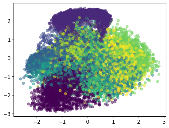
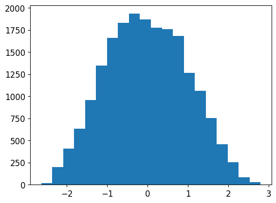
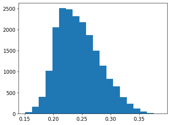
6.6 仅使用重建损失从任务 1 和 2 训练 VAE Train VAE from Task 1 and 2 only with Reconstruction loss
1
2
3
4
5
6
7
8
9
10
11
12
13
14
15
16
17
18
# Create the network
rng = np.random.RandomState(seed=SEED)
vae_2 = VAE(rng=rng,
            D_in=H_height*W_width,
            D_hid_enc=256,
            D_bottleneck=2,
            D_hid_dec=256)
# Start training
unsupervised_training_VAE(vae_2,
                          vae_loss,
                          lambda_rec=1.0,
                          lambda_reg=0.0,  # <------- No regularization loss. Just reconstruction.
                          rng=rng,
                          train_imgs_all=train_imgs_flat,
                          batch_size=40,
                          learning_rate=3e-3,
                          total_iters=1000,
                          iters_per_recon_plot=50)
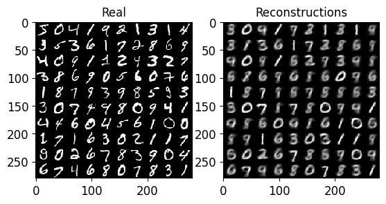
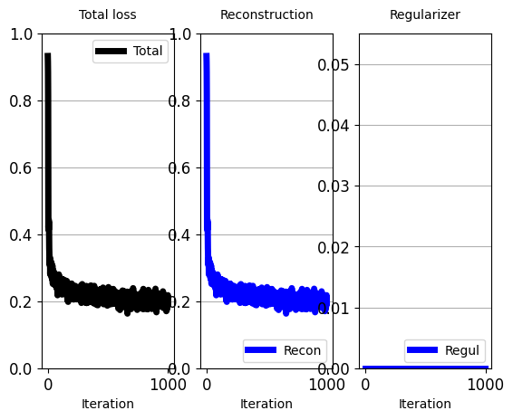
1
2
3
4
5
6
7
8
# Encode and plot
encode_training_images(vae_2, # The second VAE, trained only with Reconstruction loss.
                       train_imgs_flat,
                       train_lbls,
                       batch_size=100,
                       total_iterations=200,
                       plot_2d_embedding=True,
                       plot_hist_mu_std_for_dim=0)
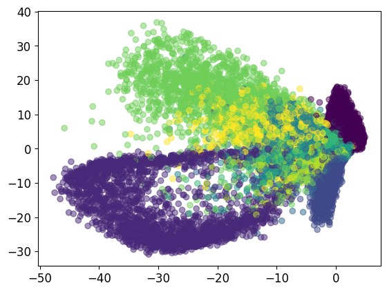
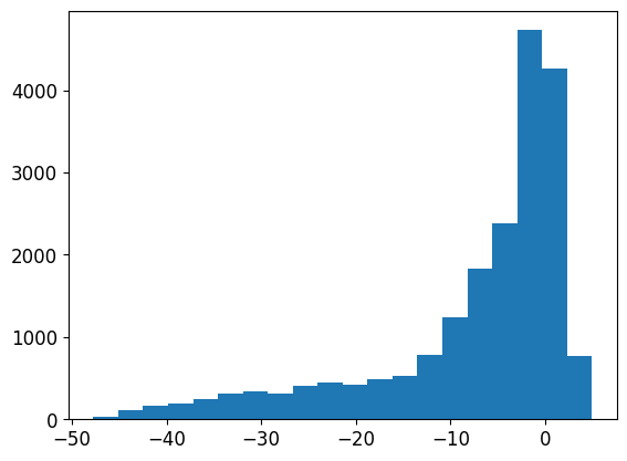
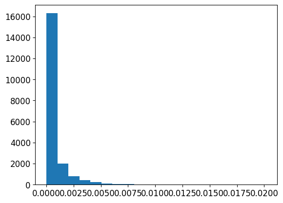
6.7 从任务 1 和 2 训练 VAE 以仅最小化正则化器 Train VAE from Task 1 and 2 to minimize only the Regularizer
1
2
3
4
5
6
7
8
9
10
11
12
13
14
15
16
17
18
# Create the network
rng = np.random.RandomState(seed=SEED)
vae_3 = VAE(rng=rng,
            D_in=H_height*W_width,
            D_hid_enc=256,
            D_bottleneck=2,
            D_hid_dec=256)
# Start training
unsupervised_training_VAE(vae_3,
                          vae_loss,
                          lambda_rec=0.0,  # <------- No reconstruction loss. Only regularizer
                          lambda_reg=0.005,
                          rng=rng,
                          train_imgs_all=train_imgs_flat,
                          batch_size=40,
                          learning_rate=3e-3,
                          total_iters=1000,
                          iters_per_recon_plot=50)
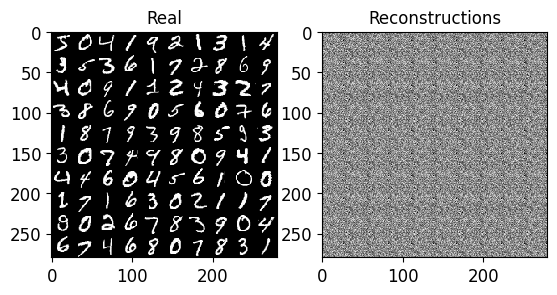
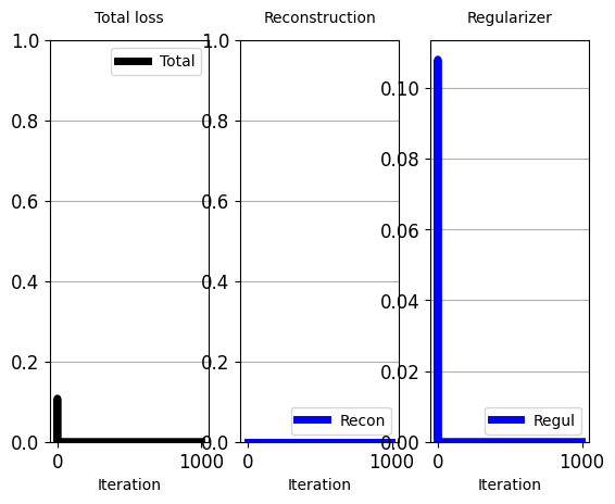
1
2
3
4
5
6
7
8
# Encode and plot
encode_training_images(vae_3, # The second VAE, trained only with Reconstruction loss.
                       train_imgs_flat,
                       train_lbls,
                       batch_size=100,
                       total_iterations=200,
                       plot_2d_embedding=True,
                       plot_hist_mu_std_for_dim=0)
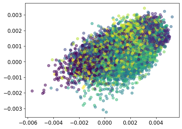
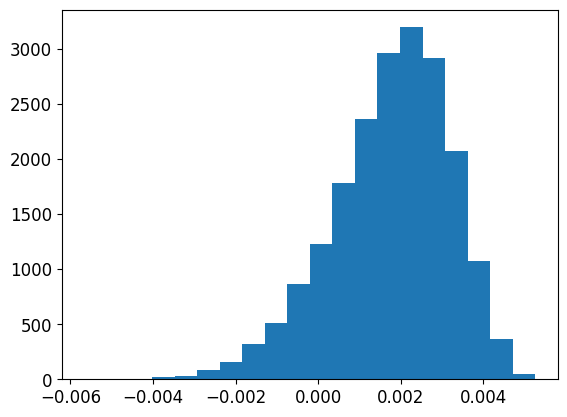
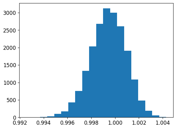
6.8 训练具有更大瓶颈层的 VAE Train a VAE with a larger bottleneck layer
1
2
3
4
5
6
7
8
9
10
11
12
13
14
15
16
17
18
19
20
21
# Same as in Task 2, but using a bottle neck with 32 dimension

# Create the network
rng = np.random.RandomState(seed=SEED)
vae_wide = VAE(rng=rng,
          D_in=H_height*W_width,
          D_hid_enc=256,
          D_bottleneck=32,  # <-----------------------------------
          D_hid_dec=256)
# Start training
unsupervised_training_VAE(vae_wide,
                          vae_loss,
                          1.0,  # alpha on the recon loss.
                          0.005,  # 0.005 works well for synthesis! 0.0005 better for smooth z values for 32n.
                          rng,
                          train_imgs_flat,
                          batch_size=40,
                          learning_rate=3e-3,  # 3e-3
                          total_iters=1000,
                          iters_per_recon_plot=50)
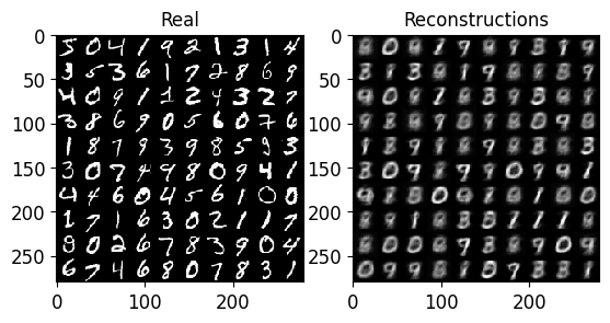
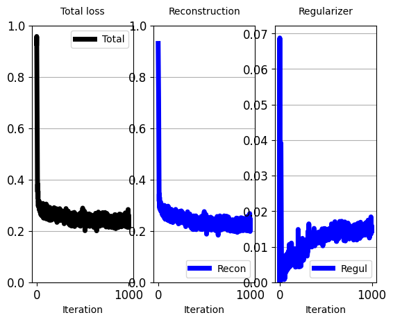
6.9 使用 VAE 合成(生成)新数据 Synthesizing (generating) new data with a VAE
1
2
3
4
5
6
7
8
9
10
11
12
13
14
15
16
17
18
19
20
21
22
23
24
25
26
27
28
def synthesize(enc_dec_net,
               rng,
               n_samples):
    # enc_dec_net: Network with encoder and decoder, pretrained.
    # n_samples: how many samples to produce.

    z_dims = enc_dec_net.D_bottleneck  # Dimensionality of z codes (and input to decoder).

    ############################## TODO: Fill in the blanks #############################
    # Create samples of z from Gaussian N(0,I), where means are 0 and standard deviations are 1 in all dimensions.
    z_samples = np.random.normal(loc=0.0, scale=1.0, size=[n_samples, z_dims])
    #####################################################################################

    z_samples_t = torch.tensor(z_samples, dtype=torch.float)
    x_samples = enc_dec_net.decode(z_samples_t)

    x_samples_np = x_samples if type(x_samples) is np.ndarray else x_samples.detach().numpy()  # torch to numpy

    for x_sample in x_samples_np:
        plot_image(x_sample.reshape([H_height, W_width]))


# Lets finally run the synthesis and see what happens...
rng = np.random.RandomState(seed=SEED)

synthesize(vae_wide,
           rng,
           n_samples=20)
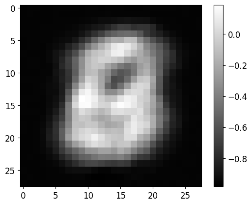
6.10 对于给定的 x,根据预测的后验 p(z|x) 重建随机样本 For a given x, reconstruct random samples from the predicted posterior p(z|x)
1
2
3
4
5
6
7
8
9
10
11
12
13
14
15
16
17
18
19
20
21
22
23
24
25
26
27
28
29
30
31
32
33
34
35
36
37
38
39
40
41
42
43
44
45
46
47
48
49
50
def sample_variations_of_x(enc_dec_net,
                           imgs_flat,
                           idx_img_x,
                           rng,
                           n_samples):
    # enc_dec_net: Network with encoder and decoder, pretrained.
    # imgs_flat:
    # idx_img_x:
    # n_samples: how many samples to produce.

    # 从图像数据集中提取索引为idx_img_x的图像,只取一个样本。
    img_x_nparray = imgs_flat[idx_img_x:idx_img_x+1]  # Shape: [num samples = 1, H * W]

    # Encode:使用VAE的编码器将图像编码到潜在空间的均值和对数标准差。
    z_mu, z_logstd = enc_dec_net.encode(img_x_nparray)  # expects array shape [N, dims_z]

    z_dims = z_mu.shape[1]  # Dimensionality of z codes (and input to decoder).
    z_mu = z_mu.detach().numpy()  # Maky pytorch tensor a numpy
    z_logstd = z_logstd.detach().numpy()

    ############# TODO: Fill in the blanks ##################################
    # Samples z values from the predicted probability of z for this sample x: p(z|x) = N(mu(x), std^2(x))
    z_std = np.exp(z_logstd)   # <------------------------------------------------------------------
    z_samples = np.random.normal(loc=z_mu, scale=z_std, size=[n_samples, z_dims]) #<------------------
    #########################################################################

    x_samples = enc_dec_net.decode(z_samples)

    x_samples_np = x_samples if type(x_samples) is np.ndarray else x_samples.detach().numpy()  # torch to numpy

    print("Real input to encoder:")
    plot_image(img_x_nparray.reshape([H_height, W_width]))
    print("Reconstructions based on samples from p(z|x=input):")
    plot_grid_of_images(x_samples_np.reshape([n_samples, H_height, W_width]),
                        n_imgs_per_row=10,
                        dynamically=False)
    print("Going to plot all the reconstructed variations one by one, for easier visual investigation:")
    for x_sample in x_samples_np:
        plot_image(x_sample.reshape([H_height, W_width]))

    diff = img_x_nparray[0] - x_samples_np[0]

# Lets finally run the synthesis and see what happens...
rng = np.random.RandomState(seed=SEED)

sample_variations_of_x(vae_wide,  # The VAE with 32 dimensional Z.
                       train_imgs_flat,
                       idx_img_x=1,  # We will encode the image with index 1, and then reconstruct it.
                       rng=rng,
                       n_samples=100)
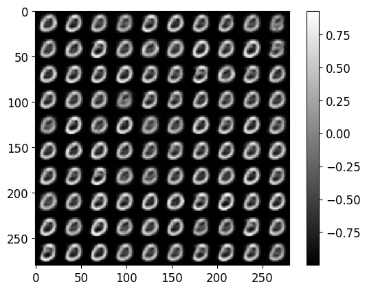
6.11 在空间 Z 中的 x_1 和 x_2 之间进行插值 Interpolate between x_1 and x_2 in space Z
1
2
3
4
5
6
7
8
9
10
11
12
13
14
15
16
17
18
19
20
21
22
23
24
25
26
27
28
29
30
31
32
33
34
35
36
37
38
39
40
41
42
43
44
45
46
47
48
49
50
51
52
53
54
55
56
57
58
59
60
61
62
63
64
def interpolate_between_x1_x2(enc_dec_net,
                              imgs_flat,
                              idx_x1,
                              idx_x2,
                              rng):
    # enc_dec_net: Network with encoder and decoder, pretrained.
    # imgs_flat: [number of images, H * W]
    # idx_x1: index of x1: x1 = imgs_flat[idx_x1]
    # idx_x2: index of x2: x2 = imgs_flat[idx_x2]
    # n_samples: how many samples to produce.

    img_x1_nparray = imgs_flat[idx_x1]
    img_x2_nparray = imgs_flat[idx_x2]
    z_mus, z_logstds = enc_dec_net.encode(np.array([img_x1_nparray, img_x2_nparray]))
    z_mus = z_mus.detach().numpy()

    z_mu1 = z_mus[0]  # np vector with [z-dims] elements
    z_mu2 = z_mus[1]

    z_dims = z_mu1.shape[0]  # Dimensionality of z codes (and input to decoder).

    # Reconstruct x1 and x2 based on mu codes:
    x_samples = enc_dec_net.decode(np.array([z_mu1, z_mu2]))
    x_samples = x_samples.detach().numpy()
    x1_rec = x_samples[0]
    x2_rec = x_samples[1]

    # Interpolate:
    alphas = [0.0, 0.1, 0.2, 0.3, 0.4, 0.5, 0.6, 0.7, 0.8, 0.9, 1.0]

    alphas_np = np.ones([11, z_dims], dtype="float16")  # [number of interpolated samples = 11, z-dimensions]
    for row_idx in range(alphas_np.shape[0]):
        alphas_np[row_idx] = alphas_np[row_idx] * alphas[row_idx]  # now whole 1st row == 0.0, 2nd row == 0.1, ...

    # Interpolate new z values
    zs_to_decode = z_mu1 + alphas_np * (z_mu2 - z_mu1)

    x_samples= enc_dec_net.decode(zs_to_decode)

    x_samples_np = x_samples if type(x_samples) is np.ndarray else x_samples.detach().numpy()  # torch to numpy

    print("Inputs to encoder:")
    plot_images([img_x1_nparray.reshape([H_height, W_width]), img_x2_nparray.reshape([H_height, W_width])],
               titles=["Real x1", "Real x2"])
    print("Reconstructions of x1 and x2 based on their most likely predicted z codes (corresponding mus):")
    plot_images([x1_rec.reshape([H_height, W_width]), x2_rec.reshape([H_height, W_width])],
               titles=["Recon of x1", "Recon of x2"])
    print("Decodings based on z samples interpolated between mu(x1) and mu(x2) predicted by encoder:")
    plot_grid_of_images(x_samples_np.reshape([11, H_height, W_width]),
                        n_imgs_per_row=11,
                        dynamically=False)
    print("Going to plot all the reconstructed variations one by one, for easier visual investigation:")
    for x_sample in x_samples_np:
        plot_image(x_sample.reshape([H_height, W_width]))


# Lets finally run the synthesis and see what happens...
rng = np.random.RandomState(seed=SEED)

interpolate_between_x1_x2(vae_wide,
                          train_imgs_flat,
                          idx_x1=1,
                          idx_x2=3,
                          rng=rng)
6.12 使用 VAE 从未标记数据中学习,以在标记数据有限时补充监督分类器:让我们首先“从头开始”训练一个监督分类器 Learning from Unlabelled data with a VAE, to complement Supervised Classifier when Labelled data are limited: Lets first train a supervised Classifier ‘from scratch’
1
2
3
4
5
6
7
8
9
10
11
12
13
14
15
16
17
18
19
20
21
22
23
24
25
26
27
28
29
30
31
32
33
34
35
36
37
38
39
40
41
42
43
44
45
46
47
48
49
50
51
52
53
54
55
56
57
58
59
60
61
62
63
64
65
66
67
68
69
70
71
72
73
74
75
76
77
78
79
80
81
82
83
84
85
86
87
88
89
90
91
92
93
94
95
96
97
98
99
100
101
102
103
104
105
106
107
108
109
110
111
112
113
114
115
116
117
118
119
120
121
122
123
124
125
126
127
128
129
130
131
132
133
134
135
136
137
138
139
140
141
142
143
144
145
146
147
148
149
150
151
152
153
154
155
156
157
158
159
160
161
162
163
164
165
166
167
168
169
class Classifier_3layers(Network):
    def __init__(self, D_in, D_hid_1, D_hid_2, D_out, rng):
        D_in = D_in
        D_hid_1 = D_hid_1
        D_hid_2 = D_hid_2
        D_out = D_out

        # === NOTE: Notice that this is exactly the same architecture as encoder of AE in Task 4 ====
        w_1_init = rng.normal(loc=0.0, scale=0.01, size=(D_in+1, D_hid_1))
        w_2_init = rng.normal(loc=0.0, scale=0.01, size=(D_hid_1+1, D_hid_2))
        w_out_init = rng.normal(loc=0.0, scale=0.01, size=(D_hid_2+1, D_out))

        w_1 = torch.tensor(w_1_init, dtype=torch.float, requires_grad=True)
        w_2 = torch.tensor(w_2_init, dtype=torch.float, requires_grad=True)
        w_out = torch.tensor(w_out_init, dtype=torch.float, requires_grad=True)

        self.params = [w_1, w_2, w_out]


    def forward_pass(self, batch_inp):
        # compute predicted y
        [w_1, w_2, w_out] = self.params

        # In case input is image, make it a tensor.
        batch_imgs_t = torch.tensor(batch_inp, dtype=torch.float) if type(batch_inp) is np.ndarray else batch_inp

        unary_feature_for_bias = torch.ones(size=(batch_imgs_t.shape[0], 1)) # [N, 1] column vector.
        x = torch.cat((batch_imgs_t, unary_feature_for_bias), dim=1) # Extra feature=1 for bias.

        # === NOTE: This is the same architecture as encoder of AE in Task 4, with extra classification layer ===
        # Layer 1
        h1_preact = x.mm(w_1)
        h1_act = h1_preact.clamp(min=0)
        # Layer 2 (corresponds to bottleneck of the AE):
        h1_ext = torch.cat((h1_act, unary_feature_for_bias), dim=1)
        h2_preact = h1_ext.mm(w_2)
        h2_act = h2_preact.clamp(min=0)
        # Output classification layer
        h2_ext = torch.cat((h2_act, unary_feature_for_bias), dim=1)
        h_out = h2_ext.mm(w_out)

        logits = h_out

        # === Addition of a softmax function for
        # Softmax activation function.
        exp_logits = torch.exp(logits)
        y_pred = exp_logits / torch.sum(exp_logits, dim=1, keepdim=True)
        # sum with Keepdim=True returns [N,1] array. It would be [N] if keepdim=False.
        # Torch broadcasts [N,1] to [N,D_out] via repetition, to divide elementwise exp_h2 (which is [N,D_out]).

        return y_pred


def cross_entropy(y_pred, y_real, eps=1e-7):
    # y_pred: Predicted class-posterior probabilities, returned by forward_pass. Numpy array of shape [N, D_out]
    # y_real: One-hot representation of real training labels. Same shape as y_pred.

    # If number array is given, change it to a Torch tensor.
    y_pred = torch.tensor(y_pred, dtype=torch.float) if type(y_pred) is np.ndarray else y_pred
    y_real = torch.tensor(y_real, dtype=torch.float) if type(y_real) is np.ndarray else y_real

    x_entr_per_sample = - torch.sum( y_real*torch.log(y_pred+eps), dim=1)  # Sum over classes, axis=1

    loss = torch.mean(x_entr_per_sample, dim=0) # Expectation of loss: Mean over samples (axis=0).
    return loss


from utils.plotting import plot_train_progress_2

def train_classifier(classifier,
                     pretrained_VAE,
                     loss_func,
                     rng,
                     train_imgs,
                     train_lbls,
                     test_imgs,
                     test_lbls,
                     batch_size,
                     learning_rate,
                     total_iters,
                     iters_per_test=-1):
    # Arguments:
    # classifier: A classifier network. It will be trained by this function using labelled data.
    #             Its input will be either original data (if pretrained_VAE=0), ...
    #             ... or the output of the feature extractor if one is given.
    # pretrained_VAE: A pretrained AutoEncoder that will *not* be trained here.
    #      It will be used to encode input data.
    #      The classifier will take as input the output of this feature extractor.
    #      If pretrained_VAE = None: The classifier will simply receive the actual data as input.
    # train_imgs: Vectorized training images
    # train_lbls: One hot labels
    # test_imgs: Vectorized testing images, to compute generalization accuracy.
    # test_lbls: One hot labels for test data.
    # batch_size: batch size
    # learning_rate: come on...
    # total_iters: how many SGD iterations to perform.
    # iters_per_test: We will 'test' the model on test data every few iterations as specified by this.

    values_to_plot = {'loss':[], 'acc_train': [], 'acc_test': []}

    optimizer = optim.Adam(classifier.params, lr=learning_rate)

    for t in range(total_iters):
        # Sample batch for this SGD iteration
        train_imgs_batch, train_lbls_batch = get_random_batch(train_imgs, train_lbls, batch_size, rng)

        # Forward pass
        if pretrained_VAE is None:
            inp_to_classifier = train_imgs_batch
        else:
            ############### TODO FOR TASK-11 #########################################
            # FILL IN THE BLANK, to provide as input to the classifier the predicted MEAN of p(z|x) for each x.
            # Why? Because the mean is the most likely (probable) code z for x!!
            #
            z_codes_mu, z_codes_logstd = pretrained_VAE.encode(train_imgs_batch)  # AE encodes. Output will be given to Classifier
            inp_to_classifier = z_codes_mu  # <---------------------------- z_codes_???????
            ############################################################################

        y_pred = classifier.forward_pass(inp_to_classifier)

        # Compute loss:
        y_real = train_lbls_batch
        loss = loss_func(y_pred, y_real)  # Cross entropy

        # Backprop and updates.
        optimizer.zero_grad()
        grads = classifier.backward_pass(loss)
        optimizer.step()


        # ==== Report training loss and accuracy ======
        # y_pred and loss can be either np.array, or torch.tensor (see later). If tensor, make it np.array.
        y_pred_numpy = y_pred if type(y_pred) is np.ndarray else y_pred.detach().numpy()
        y_pred_lbls = np.argmax(y_pred_numpy, axis=1) # y_pred is soft/probability. Make it a hard one-hot label.
        y_real_lbls = np.argmax(y_real, axis=1)

        acc_train = np.mean(y_pred_lbls == y_real_lbls) * 100. # percentage

        loss_numpy = loss if type(loss) is type(float) else loss.item()
        if t%10 == 0:
            print("[iter:", t, "]: Training Loss: {0:.2f}".format(loss), "\t Accuracy: {0:.2f}".format(acc_train))

        # =============== Every few iterations, test accuracy ================#
        if t==total_iters-1 or t%iters_per_test == 0:
            if pretrained_VAE is None:
                inp_to_classifier_test = test_imgs
            else:
                z_codes_test_mu, z_codes_test_logstd = pretrained_VAE.encode(test_imgs)
                inp_to_classifier_test = z_codes_test_mu

            y_pred_test = classifier.forward_pass(inp_to_classifier_test)

            # ==== Report test accuracy ======
            y_pred_test_numpy = y_pred_test if type(y_pred_test) is np.ndarray else y_pred_test.detach().numpy()

            y_pred_lbls_test = np.argmax(y_pred_test_numpy, axis=1)
            y_real_lbls_test = np.argmax(test_lbls, axis=1)
            acc_test = np.mean(y_pred_lbls_test == y_real_lbls_test) * 100.
            print("\t\t\t\t\t\t\t\t Testing Accuracy: {0:.2f}".format(acc_test))

            # Keep list of metrics to plot progress.
            values_to_plot['loss'].append(loss_numpy)
            values_to_plot['acc_train'].append(acc_train)
            values_to_plot['acc_test'].append(acc_test)

    # In the end of the process, plot loss accuracy on training and testing data.
    plot_train_progress_2(values_to_plot['loss'], values_to_plot['acc_train'], values_to_plot['acc_test'], iters_per_test)
1
2
3
4
5
6
7
8
9
10
11
12
13
14
15
16
17
18
19
20
21
22
23
# Train Classifier from scratch (initialized randomly)

# Create the network
rng = np.random.RandomState(seed=SEED)
net_classifier_from_scratch = Classifier_3layers(D_in=H_height*W_width,
                                                 D_hid_1=256,
                                                 D_hid_2=32,
                                                 D_out=C_classes,
                                                 rng=rng)
# Start training
train_classifier(net_classifier_from_scratch,
                 None,  # No pretrained AE
                 cross_entropy,
                 rng,
                 train_imgs_flat[:100],
                 train_lbls_onehot[:100],
                 test_imgs_flat,
                 test_lbls_onehot,
                 batch_size=40,
                 learning_rate=3e-3,
                 total_iters=1000,
                 iters_per_test=20)
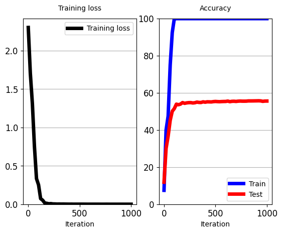
6.13 当标签有限时,使用预训练的 VAE 作为监督分类器的“特征提取器” Use pre-trained VAE as ‘feature-extractor’ for supervised Classifier when labels are limited
1
2
3
4
5
6
7
8
9
10
11
12
13
14
15
16
17
18
19
20
21
22
23
24
25
26
27
28
29
30
31
32
33
34
35
36
37
38
39
40
41
42
43
44
45
46
47
48
49
50
51
52
53
54
55
56
# Train classifier on top of pre-trained AE encoder

class Classifier_1layer(Network):
    # Classifier with just 1 layer, the classification layer
    def __init__(self, D_in, D_out, rng):
        # D_in: dimensions of input
        # D_out: dimension of output (number of classes)

        w_out_init = rng.normal(loc=0.0, scale=0.01, size=(D_in+1, D_out))
        w_out = torch.tensor(w_out_init, dtype=torch.float, requires_grad=True)
        self.params = [w_out]


    def forward_pass(self, batch_inp):
        # compute predicted y
        [w_out] = self.params

        # In case input is image, make it a tensor.
        batch_inp_t = torch.tensor(batch_inp, dtype=torch.float) if type(batch_inp) is np.ndarray else batch_inp

        unary_feature_for_bias = torch.ones(size=(batch_inp_t.shape[0], 1)) # [N, 1] column vector.
        batch_inp_ext = torch.cat((batch_inp_t, unary_feature_for_bias), dim=1) # Extra feature=1 for bias.

        # Output classification layer
        logits = batch_inp_ext.mm(w_out)

        # Output layer activation function
        # Softmax activation function.
        exp_logits = torch.exp(logits)
        y_pred = exp_logits / torch.sum(exp_logits, dim=1, keepdim=True)
        # sum with Keepdim=True returns [N,1] array. It would be [N] if keepdim=False.
        # Torch broadcasts [N,1] to [N,D_out] via repetition, to divide elementwise exp_h2 (which is [N,D_out]).

        return y_pred


# Create the network
rng = np.random.RandomState(seed=SEED) # Random number generator
# As input, it will be getting z-codes from the AE with 32-neurons bottleneck from Task 4.
classifier_1layer = Classifier_1layer(vae_wide.D_bottleneck,  # Input dimension is dimensions of AE's Z
                                      C_classes,
                                      rng=rng)

train_classifier(classifier_1layer,
                 vae_wide,  # Pretrained AE, to use as feature extractor.
                 cross_entropy,
                 rng,
                 train_imgs_flat[:100],
                 train_lbls_onehot[:100],
                 test_imgs_flat,
                 test_lbls_onehot,
                 batch_size=40,
                 learning_rate=3e-3,
                 total_iters=1000,
                 iters_per_test=20)
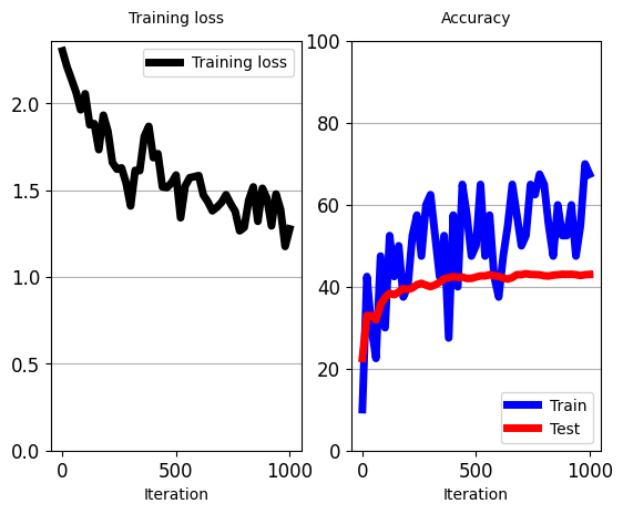
6.14 使用 VAE 编码器的参数来初始化监督分类器的权重,然后使用有限的标签进行细化 Use parameters of VAE’s encoder to initialize weights of a supervised Classifier, followed by refine ment using limited labels
1
2
3
4
5
6
7
8
9
10
11
12
13
14
15
16
17
18
19
20
21
22
23
24
25
26
27
28
29
30
31
32
33
34
35
36
37
38
39
40
41
42
43
44
45
46
47
48
# Pre-train a classifier.

# The below classifier has THE SAME architecture as the 3-layer Classifier that we trained...
# ... in a purely supervised manner in Task-10.
# This is done by inheriting the class (Classifier_3layers), therefore uses THE SAME forward_pass() function.
# THE ONLY DIFFERENCE is in the construction __init__.
# This 'pretrained' classifier receives as input a pretrained autoencoder (pretrained_VAE) from Task 6.
# It then uses the parameters of the AE's encoder to initialize its own parameters, rather than random initialization.
# The model is then trained all together.
class Classifier_3layers_pretrained(Classifier_3layers):
    def __init__(self, pretrained_VAE, D_in, D_out, rng):
        D_in = D_in
        D_hid_1 = 256
        D_hid_2 = 32
        D_out = D_out

        w_out_init = rng.normal(loc=0.0, scale=0.01, size=(D_hid_2+1, D_out))

        [vae_w1, vae_w2_mu, vae_w2_std, vae_w3, vae_w4] = pretrained_VAE.params  # Pre-trained parameters of pre-trained VAE.

        w_1 = torch.tensor(vae_w1, dtype=torch.float, requires_grad=True)
        w_2 = torch.tensor(vae_w2_mu, dtype=torch.float, requires_grad=True)
        w_out = torch.tensor(w_out_init, dtype=torch.float, requires_grad=True)

        self.params = [w_1, w_2, w_out]

# Create the network
rng = np.random.RandomState(seed=SEED) # Random number generator
classifier_3layers_pretrained = Classifier_3layers_pretrained(vae_wide,  # The AE pre-trained in Task 4.
                                                              train_imgs_flat.shape[1],
                                                              C_classes,
                                                              rng=rng)

# Start training
# NOTE: Only the 3-layer pretrained classifier is used, and will be trained all together.
# No frozen feature extractor.
train_classifier(classifier_3layers_pretrained,  # classifier that will be trained.
                 None,  # No pretrained AE to act as 'frozen' feature extractor.
                 cross_entropy,
                 rng,
                 train_imgs_flat[:100],
                 train_lbls_onehot[:100],
                 test_imgs_flat,
                 test_lbls_onehot,
                 batch_size=40,
                 learning_rate=3e-3,
                 total_iters=1000,
                 iters_per_test=20)
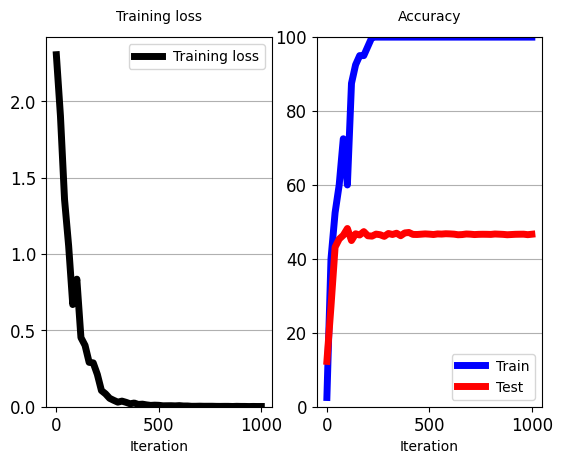
7. 生成对抗网络 Generative Adversarial Networks(GANs)
7.1 加载并刷新 MNIST Loading and Refresshing MNIST
1
2
3
4
5
6
7
8
9
10
11
12
13
14
15
16
17
18
19
20
21
22
23
24
25
26
27
28
29
# -*- coding: utf-8 -*-
# The below is for auto-reloading external modules after they are changed, such as those in ./utils.
# Issue: https://stackoverflow.com/questions/1907993/autoreload-of-modules-in-ipython
%load_ext autoreload
%autoreload 2

import numpy as np
from utils.data_utils import get_mnist # Helper function. Use it out of the box.

# Constants
DATA_DIR = './data/mnist' # Location we will keep the data.
SEED = 111111

# If datasets are not at specified location, they will be downloaded.
train_imgs, train_lbls = get_mnist(data_dir=DATA_DIR, train=True, download=True)
test_imgs, test_lbls = get_mnist(data_dir=DATA_DIR, train=False, download=True)

print("[train_imgs] Type: ", type(train_imgs), "|| Shape:", train_imgs.shape, "|| Data type: ", train_imgs.dtype )
print("[train_lbls] Type: ", type(train_lbls), "|| Shape:", train_lbls.shape, "|| Data type: ", train_lbls.dtype )
print('Class labels in train = ', np.unique(train_lbls))

print("[test_imgs] Type: ", type(test_imgs), "|| Shape:", test_imgs.shape, " || Data type: ", test_imgs.dtype )
print("[test_lbls] Type: ", type(test_lbls), "|| Shape:", test_lbls.shape, " || Data type: ", test_lbls.dtype )
print('Class labels in test = ', np.unique(test_lbls))

N_tr_imgs = train_imgs.shape[0] # N hereafter. Number of training images in database.
H_height = train_imgs.shape[1] # H hereafter
W_width = train_imgs.shape[2] # W hereafter
C_classes = len(np.unique(train_lbls)) # C hereafter
1
2
3
%matplotlib inline
from utils.plotting import plot_grid_of_images # Helper functions, use out of the box.
plot_grid_of_images(train_imgs[0:100], n_imgs_per_row=10)
7.2 数据预处理 Data pre-processing
1
2
3
4
5
6
7
# a) Change representation of labels to one-hot vectors of length C=10.
train_lbls_onehot = np.zeros(shape=(train_lbls.shape[0], C_classes ) )
train_lbls_onehot[ np.arange(train_lbls_onehot.shape[0]), train_lbls ] = 1
test_lbls_onehot = np.zeros(shape=(test_lbls.shape[0], C_classes ) )
test_lbls_onehot[ np.arange(test_lbls_onehot.shape[0]), test_lbls ] = 1
print("BEFORE: [train_lbls]        Type: ", type(train_lbls), "|| Shape:", train_lbls.shape, " || Data type: ", train_lbls.dtype )
print("AFTER : [train_lbls_onehot] Type: ", type(train_lbls_onehot), "|| Shape:", train_lbls_onehot.shape, " || Data type: ", train_lbls_onehot.dtype )
1
2
3
4
5
6
7
8
9
10
11
12
13
14
15
16
# b) Re-scale image intensities, from [0,255] to [-1, +1].
# This commonly facilitates learning:
# A zero-centered signal with small magnitude allows avoiding exploding/vanishing problems easier.
from utils.data_utils import normalize_int_whole_database # Helper function. Use out of the box.
train_imgs = normalize_int_whole_database(train_imgs, norm_type="minus_1_to_1")
test_imgs = normalize_int_whole_database(test_imgs, norm_type="minus_1_to_1")

# Lets plot one image.
from utils.plotting import plot_image, plot_images # Helper function, use out of the box.
index = 0  # Try any, up to 60000
print("Plotting image of index: [", index, "]")
print("Class label for this image is: ", train_lbls[index])
print("One-hot label representation: [", train_lbls_onehot[index], "]")
plot_image(train_imgs[index])
# Notice the magnitude of intensities. Black is now negative and white is positive float.
# Compare with intensities of figure further above.
1
2
3
4
5
6
# c) Flatten the images, from 2D matrices to 1D vectors. MLPs take feature-vectors as input, not 2D images.
train_imgs_flat = train_imgs.reshape([train_imgs.shape[0], -1]) # Preserve 1st dim (S = num Samples), flatten others.
test_imgs_flat = test_imgs.reshape([test_imgs.shape[0], -1])
print("Shape of numpy array holding the training database:")
print("Original : [N, H, W] = [", train_imgs.shape , "]")
print("Flattened: [N, H*W]  = [", train_imgs_flat.shape , "]")
7.3 实施 GAN Implementing a GAN
1
2
3
4
5
6
7
8
9
10
11
12
13
14
15
16
17
18
19
20
21
22
23
24
25
26
27
28
29
30
31
32
33
34
35
36
37
38
39
40
41
42
43
44
45
46
47
48
49
50
51
52
53
54
55
56
57
58
59
60
61
62
63
64
65
66
67
68
69
70
71
72
73
74
75
76
77
78
79
80
81
82
83
84
85
86
87
88
89
90
91
92
93
94
95
96
97
98
99
100
101
102
103
104
105
106
107
108
109
110
111
112
113
114
115
116
117
118
119
120
121
122
123
124
125
126
127
128
129
130
131
132
133
134
135
136
137
138
139
140
141
142
143
# -*- coding: utf-8 -*-
import torch
import torch.optim as optim
import torch.nn as nn

lrelu = nn.LeakyReLU(0.2)

class Network():

    def backward_pass(self, loss):
        # Performs back propagation and computes gradients
        # With PyTorch, we do not need to compute gradients analytically for parameters were requires_grads=True,
        # Calling loss.backward(), torch's Autograd automatically computes grads of loss wrt each parameter p,...
        # ... and **puts them in p.grad**. Return them in a list.
        loss.backward()
        grads = [param.grad for param in self.params]
        return grads


class Generator(Network):
    def __init__(self, rng, D_z, D_hid1, D_hid2, D_data):
        self.D_z = D_z  # Keep track of it, we may need it.
        # Initialize weight matrices
        # Dimensions of parameter tensors are (number of neurons + 1) per layer, to account for +1 bias.
        # First 2 hidden layers 随机生成
        w1_init = rng.normal(loc=0.0, scale=np.sqrt(2./(D_z * D_hid1)), size=(D_z + 1, D_hid1))
        w2_init = rng.normal(loc=0.0, scale=np.sqrt(2./(D_hid1 * D_hid2)), size=(D_hid1 + 1, D_hid2))
        # -- Output layer, predicting p(real|x)
        wout_init = rng.normal(loc=0.0, scale=np.sqrt(2./(D_hid2 * D_data)), size=(D_hid2 + 1, D_data))

        # Pytorch tensors, parameters of the model
        # Use the above numpy arrays as of random floats as initialization for the Pytorch weights.
        w1 = torch.tensor(w1_init, dtype=torch.float, requires_grad=True)
        w2 = torch.tensor(w2_init, dtype=torch.float, requires_grad=True)
        wout = torch.tensor(wout_init, dtype=torch.float, requires_grad=True)

        # Keep track of all trainable parameters:
        self.params = [w1, w2, wout]


    def forward(self, batch_z):
        # z_codes: numpy array or pytorch tensor, shape [N, dimensionality of data]
        [w1, w2, wout] = self.params
        # make numpy to pytorch tensor
        batch_z_t = torch.tensor(batch_z, dtype=torch.float) if type(batch_z) is np.ndarray else batch_z
        # add 1 element for bias
        unary_feature_for_bias = torch.ones(size=(batch_z_t.shape[0], 1))  # [N, 1] column vector.

        # ========== TODO: Fill in the gaps ========
        # hidden layer:
        z_ext = torch.cat((batch_z_t, unary_feature_for_bias), dim=1)
        h1_preact = z_ext.mm(w1)
        h1_act = lrelu(h1_preact)
        # l2
        h1_ext = torch.cat((h1_act, unary_feature_for_bias), dim=1)
        h2_preact = h1_ext.mm(w2)
        h2_act = lrelu(h2_preact)
        # output layer.
        h2_ext = torch.cat((h2_act, unary_feature_for_bias), dim=1)
        hout_preact = h2_ext.mm(wout)
        hout_act = torch.tanh(hout_preact)
        # ==========================================

        # Output
        x_generated = hout_act  # [N_samples, dimensionality of data]

        return x_generated


class Discriminator(Network):
    def __init__(self, rng, D_data, D_hid1, D_hid2):
        # Initialize weight matrices
        # Dimensions of parameter tensors are (number of neurons + 1) per layer, to account for +1 bias.
        # -- 2 hidden layers 随机生成
        w1_init = rng.normal(loc=0.0, scale=np.sqrt(2. / (D_data * D_hid1)), size=(D_data + 1, D_hid1))
        w2_init = rng.normal(loc=0.0, scale=np.sqrt(2. / (D_hid1 * D_hid2)), size=(D_hid1 + 1, D_hid2))
        # -- Output layer, predicting p(real|x)
        wout_init = rng.normal(loc=0.0, scale=np.sqrt(2. / D_hid2), size=(D_hid2 + 1, 1))

        # Pytorch tensors, parameters of the model
        # Use the above numpy arrays as of random floats as initialization for the Pytorch weights.
        w1 = torch.tensor(w1_init, dtype=torch.float, requires_grad=True)
        w2 = torch.tensor(w2_init, dtype=torch.float, requires_grad=True)
        wout = torch.tensor(wout_init, dtype=torch.float, requires_grad=True)

        # Keep track of all trainable parameters:
        self.params = [w1, w2, wout]


    def forward(self, batch_x):
        # z_codes: numpy array or pytorch tensor, shape [N, dimensionality of data]
        [w1, w2, wout] = self.params
        # make numpy to pytorch tensor
        batch_x_t = torch.tensor(batch_x, dtype=torch.float) if type(batch_x) is np.ndarray else batch_x
        # Add 1 element or bias
        unary_feature_for_bias = torch.ones(size=(batch_x_t.shape[0], 1)) # [N, 1] column vector.

        # ========== TODO: Fill in the gaps ========
        # hidden layer:
        x_ext = torch.cat((batch_x_t, unary_feature_for_bias), dim=1)
        h1_preact = x_ext.mm(w1)
        h1_act = lrelu(h1_preact)
        # layer 2
        h1_ext = torch.cat((h1_act, unary_feature_for_bias), dim=1)
        h2_preact = h1_ext.mm(w2)
        h2_act = lrelu(h2_preact)
        # output layer.
        h2_ext = torch.cat((h2_act, unary_feature_for_bias), dim=1)
        hout_preact = h2_ext.mm(wout)
        hout_act = torch.sigmoid(hout_preact)
        # ===========================================

        # Output
        p_real = hout_act

        return p_real


def generator_loss_practical(p_generated_x_is_real):
    # mu: Tensor, [number of samples]. Predicted probability D(G(z)) that fake data are real.

    ######## TODO: Complete the gap ###########
    loss_per_sample = - torch.log(p_generated_x_is_real)
    ###########################################
    expected_loss = torch.mean(loss_per_sample, dim=0) # Expectation of loss: Mean over samples (axis=0).
    return expected_loss


def discriminator_loss(p_real_x_is_real, p_generated_x_is_real):
    # p_real_x_is_real: [N] Predicted probability D(x) for x~training_data that real data are real.
    # p_generated_x_is_real: [N]. Predicted probability D(x) for x=G(z) where z~N(0,I) that fake data are real.

    ######## TODO: Complete the calculation of Reconstruction loss for each sample ###########
    loss_per_real_x = - torch.log(p_real_x_is_real)
    exp_loss_reals = torch.mean(loss_per_real_x)

    loss_per_fake_x = - torch.log(1 - p_generated_x_is_real)
    exp_loss_fakes = torch.mean(loss_per_fake_x)
    ##########################################################################################

    total_loss = exp_loss_reals + exp_loss_fakes  # Expectation of loss: Mean over samples (axis=0).
    return total_loss
7.4 实施 GAN 的无监督训练 Implement unsupervised training of a GAN
1
2
3
4
5
6
7
8
9
10
11
12
13
14
15
16
17
18
19
20
21
22
23
24
25
26
27
28
29
30
31
32
33
34
35
36
37
38
39
40
41
42
43
44
45
46
47
48
49
50
51
52
53
54
55
56
57
58
59
60
61
62
63
64
65
66
67
68
69
70
71
72
73
74
75
76
77
78
79
80
81
82
83
84
85
86
87
88
89
90
91
92
93
94
95
96
97
98
99
100
101
102
103
104
105
106
107
108
109
110
111
112
113
114
115
116
117
118
119
120
121
122
123
124
125
126
127
128
129
130
131
132
133
134
135
136
137
138
139
140
141
142
143
144
from utils.plotting import plot_train_progress_GAN, plot_grids_of_images  # Use out of the box


def get_batch_reals(train_imgs, train_lbls, batch_size, rng):
    # train_imgs: Images. Numpy array of shape [N, H * W]
    # train_lbls: Labels of images. None, or Numpy array of shape [N, C_classes], one hot label for each image.
    # batch_size: integer. Size that the batch should have.

    indices = range(0, batch_size)  # Remove this line after you fill-in and un-comment the below.
    indices = rng.randint(low=0, high=train_imgs.shape[0], size=batch_size, dtype='int32')

    train_imgs_batch = train_imgs[indices]
    if train_lbls is not None:  # Enables function to be used both for supervised and unsupervised learning
        train_lbls_batch = train_lbls[indices]
    else:
        train_lbls_batch = None
    return [train_imgs_batch, train_lbls_batch]


def unsupervised_training_GAN(generator,
                              discriminator,
                              loss_func_g,
                              loss_func_d,
                              rng,
                              train_imgs_all,
                              batch_size_g,
                              batch_size_d_fakes,
                              batch_size_d_reals,
                              learning_rate_g,
                              learning_rate_d,
                              total_iters_g,
                              inner_iters_d,
                              iters_per_gen_plot=-1):
    # generator: Instance of a Generator.
    # discriminator: Instance of a Discriminator.
    # loss_func_g: Loss functions of G
    # loss_func_d: Loss functions of D
    # rng: numpy random number generator
    # train_imgs_all: All the training images. Numpy array, shape [N_tr, H, W]
    # batch_size_g: Size of the batch for G when it is its turn to get updated.
    # batch_size_d_fakes: Size of batch of fake samples for D when it is its turn to get updated.
    # batch_size_d_reals: Size of batch of real samples for D when it is its turn to get updated.
    # learning_rate_g: Learning rate for G.
    # learning_rate_d: learning rate for D.
    # total_iters_g: how many SGD iterations to perform for G in total (outer loop).
    # inner_iters_d: how many SGD iterations to perform for D before every 1 SGD iteration of G.
    # iters_per_gen_plot: Integer. Every that many iterations the model generates few examples and we plot them.
    loss_g_to_plot = []
    loss_d_to_plot = []
    loss_g_mom_to_plot = []
    loss_d_mom_to_plot = []
    loss_g_mom = None
    loss_d_mom = None

    optimizer_g = optim.Adam(generator.params, lr=learning_rate_g, betas=[0.5, 0.999], eps=1e-07, weight_decay=0)  # Will use PyTorch's Adam optimizer out of the box
    optimizer_d = optim.Adam(discriminator.params, lr=learning_rate_d, betas=[0.5, 0.99], eps=1e-07, weight_decay=0)  # Will use PyTorch's Adam optimizer out of the box

    for t in range(total_iters_g):

        for k in range(inner_iters_d):
            # Train Discriminator for inner_iters_d SGD iterations...

            ################## TODO: Fill in the gaps #######################
            # Generate Fake samples with G
            z_batch = np.random.normal(loc=0., scale=1., size=[batch_size_d_fakes, generator.D_z])
            x_gen_batch = generator.forward(z_batch)
            # Forward pass of fake samples through D
            p_gen_x_are_real = discriminator.forward(x_gen_batch)

            # Forward pass of real samples through D
            x_reals_batch, _ = get_batch_reals(train_imgs_all, None, batch_size_d_reals, rng)
            p_real_x_are_real = discriminator.forward(x_reals_batch)

            # Compute D loss:
            loss_d = loss_func_d(p_real_x_are_real, p_gen_x_are_real)
            ####################################################################

            # Backprop to D
            optimizer_d.zero_grad()
            _ = discriminator.backward_pass(loss_d)
            optimizer_d.step()

        ############## Train Generator for 1 SGD iteration ############

        ########## TODO: Fill in the gaps ##################################
        # Generate Fake samples with G
        z_batch = np.random.normal(loc=0., scale=1., size=[batch_size_g, generator.D_z])
        x_gen_batch = generator.forward(z_batch)
        # Forward pass of fake samples through D
        p_gen_x_are_real = discriminator.forward(x_gen_batch)
        ####################################################################

        # Compute G loss:
        loss_g = loss_func_g(p_gen_x_are_real)

        # Backprop to G
        optimizer_g.zero_grad()
        _ = generator.backward_pass(loss_g)
        optimizer_g.step()

        # ==== Report training loss and accuracy ======
        loss_g_np = loss_g if type(loss_g) is type(float) else loss_g.item()
        loss_d_np = loss_d if type(loss_d) is type(float) else loss_d.item()
        if t % 10 == 0:  # Print every 10 iterations
            print("[iter:", t, "]: Loss G: {0:.2f}".format(loss_g_np), " Loss D: {0:.2f}".format(loss_d_np))

        loss_g_mom = loss_g_np if loss_g_mom is None else loss_g_mom * 0.9 + 0.1 * loss_g_np
        loss_d_mom = loss_d_np if loss_d_mom is None else loss_d_mom * 0.9 + 0.1 * loss_d_np

        loss_g_to_plot.append(loss_g_np)
        loss_d_to_plot.append(loss_d_np)
        loss_g_mom_to_plot.append(loss_g_mom)
        loss_d_mom_to_plot.append(loss_d_mom)

        # =============== Every few iterations, plot loss ================#
        if t == total_iters_g - 1 or t % iters_per_gen_plot == 0:

            ########## TODO: Fill in the gaps #############################
            # Generate Fake samples with G
            n_samples_to_gen = 100
            z_plot = np.random.normal(loc=0., scale=1., size=[100, generator.D_z])
            x_gen_plot = generator.forward(z_plot)
            # Cast tensors to numpy arrays
            x_gen_plot_np = x_gen_plot if type(x_gen_plot) is np.ndarray else x_gen_plot.detach().numpy()
            ###############################################################

            # Generated images have vector shape. Reshape them to original image shape.
            x_gen_plot_resh = x_gen_plot_np.reshape([n_samples_to_gen, H_height, W_width])

            train_imgs_resh = train_imgs_all.reshape([train_imgs_all.shape[0], H_height, W_width])


            # Plot a few generated images.
            plot_grids_of_images([x_gen_plot_resh[0:100], train_imgs_resh[0:100]],
                                  titles=["Generated", "Real"],
                                  n_imgs_per_row=10,
                                  dynamically=True)

    # In the end of the process, plot loss.
    plot_train_progress_GAN(loss_g_to_plot, loss_d_to_plot,
                            loss_g_mom_to_plot, loss_d_mom_to_plot,
                            iters_per_point=1, y_lims=[3., 3.])
7.5 实例化并训练您的 GAN Instantiate and Train your GAN
1
2
3
4
5
6
7
8
9
10
11
12
13
14
15
16
17
18
19
20
21
22
23
24
25
26
27
28
# Create the network
rng = np.random.RandomState(seed=SEED)
generator = Generator(rng=rng,
                      D_z=128,
                      D_hid1=256,
                      D_hid2=512,
                      D_data=H_height*W_width)
discriminator = Discriminator(rng=rng,
                              D_data=H_height*W_width,
                              D_hid1=256,
                              D_hid2=512)

# Start training
unsupervised_training_GAN(generator,
                          discriminator,
                          loss_func_g=generator_loss_practical,
                          loss_func_d=discriminator_loss,
                          rng=rng,
                          train_imgs_all=train_imgs_flat,
                          batch_size_g=32,
                          batch_size_d_fakes=64,
                          batch_size_d_reals=64,
                          learning_rate_g=1e-3,
                          learning_rate_d=1e-3,
                          total_iters_g=5000,
                          inner_iters_d=1,
                          iters_per_gen_plot=100)
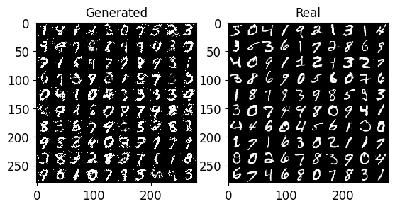
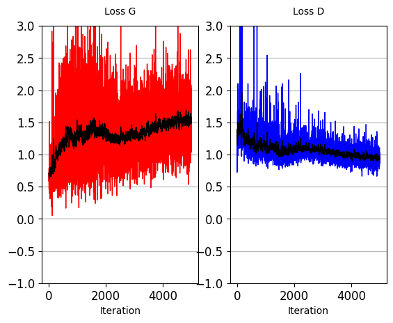
7.6 使用 GAN 生成新图像 Generate new images using your GAN
1
2
3
4
5
6
7
8
9
10
11
12
13
14
15
def synthesize(generator, n_samples):

        # Generate Fake samples with G
        z_plot = np.random.normal(loc=0., scale=1., size=[n_samples, generator.D_z])
        x_gen_plot = generator.forward(z_plot)
        # Cast tensors to numpy arrays
        x_gen_plot_np = x_gen_plot if type(x_gen_plot) is np.ndarray else x_gen_plot.detach().numpy()

        # Generated images have vector shape. Reshape them to original image shape.
        x_gen_plot_resh = x_gen_plot_np.reshape([n_samples, H_height, W_width])

        for i in range(n_samples):
            plot_image(x_gen_plot_resh[i])

synthesize(generator, 100)
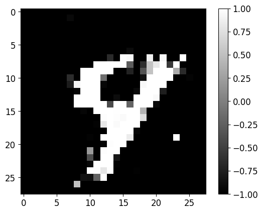
8. 循环神经网络 Recurrent Neural Networks(RNN)
8.1 示例一:使用 RNN 生成句子中的下一个单词
8.1.1 导入库
1
2
3
import torch
from torch import nn
import numpy as np
8.1.2 数据生成 Data Generation
1
2
3
4
5
6
7
8
9
10
11
12
13
text = ['hey we are teaching deep learning','hey how are you', 'have a nice day', 'nice to meet you']

# Join all the sentences together and extract the unique characters from the combined sentences
# 筛选出句子中出现的字母
chars = set(''.join(text))

# Creating a dictionary that maps integers to the characters
# 一个int 转 char的字典
int2char = dict(enumerate(chars))

# Creating another dictionary that maps characters to integers
# 一个char 转 int的字典
char2int = {char: ind for ind, char in int2char.items()}
1
2
3
4
5
6
7
8
9
10
11
12
13
14
15
16
17
18
19
20
21
22
char2int
'''
{'i': 0,
 'e': 1,
 'o': 2,
 'v': 3,
 'p': 4,
 't': 5,
 'a': 6,
 'r': 7,
 'd': 8,
 ' ': 9,
 'u': 10,
 'y': 11,
 'm': 12,
 'c': 13,
 'g': 14,
 'l': 15,
 'h': 16,
 'n': 17,
 'w': 18}
'''
1
2
3
4
5
6
7
8
9
10
11
12
# Finding the length of the longest string in our data
maxlen = len(max(text, key=len))

# Padding
# 把所有句子padding为maxlen+1的长度
# maxlen+=1 means adding a ' ' at each sentence, which helps to predict last word of sentences
maxlen+=1
# A simple loop that loops through the list of sentences and adds a ' ' whitespace until the length of
# the sentence matches the length of the longest sentence
for i in range(len(text)):
  while len(text[i])<maxlen:
      text[i] += ' '
1
2
3
4
5
6
7
8
9
10
11
# Creating lists that will hold our input and target sequences
input_seq = []
target_seq = []

for i in range(len(text)):
    # Remove last character for input sequence
  input_seq.append(text[i][:-1])

    # Remove first character for target sequence
  target_seq.append(text[i][1:])
  print("Input Sequence: {}\nTarget Sequence: {}".format(input_seq[i], target_seq[i]))
该地方应该是有bug,这里移除的是最后一位padding的空格
正确结果为:
- Input Sequence: hey how are yo
- Target Sequence: ey how are you
1
2
3
for i in range(len(text)):
    input_seq[i] = [char2int[character] for character in input_seq[i]]
    target_seq[i] = [char2int[character] for character in target_seq[i]]
8.1.3 独热编码 One-Hot Encoding
1
2
3
4
5
6
7
8
9
10
11
12
13
14
15
dict_size = len(char2int)
seq_len = maxlen - 1
batch_size = len(text)

def one_hot_encode(sequence, dict_size, seq_len, batch_size):
    # Creating a multi-dimensional array of zeros with the desired output shape
    # 创造一个多维初始化为0的数组
    features = np.zeros((batch_size, seq_len, dict_size), dtype=np.float32)

    # Replacing the 0 at the relevant character index with a 1 to represent that character
    # 替换掉对应位置为1
    for i in range(batch_size):
        for u in range(seq_len):
            features[i, u, sequence[i][u]] = 1
    return features
1
2
3
4
5
6
7
# Input shape --> (Batch Size, Sequence Length, One-Hot Encoding Size)
input_seq = one_hot_encode(input_seq, dict_size, seq_len, batch_size)
print(input_seq.shape)

'''
(4, 34, 19)
'''
1
2
input_seq = torch.from_numpy(input_seq)
target_seq = torch.Tensor(target_seq)
8.1.4 定义RNN模型 Defining RNN Model
1
2
3
4
5
6
7
8
9
10
11
12
13
14
15
16
17
18
19
20
21
22
23
24
25
26
27
28
29
30
31
32
33
34
35
36
37
38
class Model(nn.Module):
    def __init__(self, input_size, output_size, hidden_dim, n_layers):
        super(Model, self).__init__()

        # Defining some parameters
        self.hidden_dim = hidden_dim
        self.n_layers = n_layers

        #Defining the layers
        # RNN Layer
        self.rnn = nn.RNN(input_size, hidden_dim, n_layers, batch_first=True)
        # Fully connected layer
        self.fc = nn.Linear(hidden_dim, output_size)

    def forward(self, x):

        batch_size = x.size(0)

        # Initializing hidden state for first input using method defined below
        hidden = self.init_hidden(batch_size)

        # Passing in the input and hidden state into the model and obtaining outputs
        # 将输入和隐藏状态传递给 RNN 层,获取输出和更新后的隐藏状态
        out, hidden = self.rnn(x, hidden)

        # Reshaping the outputs such that it can be fit into the fully connected layer
        # 将 RNN 输出的形状重新调整,以便能够输入到全连接层
        out = out.contiguous().view(-1, self.hidden_dim)
        # 通过全连接层获取最终输出
        out = self.fc(out)

        return out, hidden

    def init_hidden(self, batch_size):
        # This method generates the first hidden state of zeros which we'll use in the forward pass
        # We'll send the tensor holding the hidden state to the device we specified earlier as well
        hidden = torch.zeros(self.n_layers, batch_size, self.hidden_dim)
        return hidden
1
2
3
4
5
6
7
8
9
10
11
# Instantiate the model with hyperparameters
model = Model(input_size=dict_size, output_size=dict_size, hidden_dim=12, n_layers=1)


# Define hyperparameters
n_epochs = 200
lr=0.01

# Define Loss, Optimizer
criterion = nn.CrossEntropyLoss()
optimizer = torch.optim.Adam(model.parameters(), lr=lr)
8.1.5 测试RNN Testing RNN
1
2
3
4
5
6
7
8
9
10
11
12
13
14
15
# This function takes in the model and character as arguments and returns the next character prediction and hidden state
def predict(model, character):
    # One-hot encoding our input to fit into the model
    character = np.array([[char2int[c] for c in character]])
    character = one_hot_encode(character, dict_size, character.shape[1], 1)
    character = torch.from_numpy(character)


    out, hidden = model(character)

    prob = nn.functional.softmax(out[-1], dim=0).data
    # Taking the class with the highest probability score from the output
    char_ind = torch.max(prob, dim=0)[1].item()

    return int2char[char_ind], hidden
1
2
3
4
5
6
7
8
9
10
11
12
13
14
15
16
def sample(model, start='hey'):
    model.eval() # eval mode
    start = start.lower()
    # First off, run through the starting characters
    chars = [ch for ch in start]
    size = maxlen
    # Now pass in the previous characters and get a new one
    c=0
    for ii in range(size):
        char, h = predict(model, chars)
        c+=1
        if char==' ' and c>1:
            break
        chars.append(char)

    return ''.join(chars)
1
2
3
4
5
6
7
8
9
10
11
12
13
14
15
16
17
18
19
sample(model, 'hey we are teaching deep')
'''
'hey we are teaching deep learning'
'''

sample(model, 'hey how are')
'''
'hey how are you'
'''

sample(model, 'nice to meet')
'''
'nice to meet you'
'''

sample(model, 'have a nice')
'''
'have a nice day'
'''
8.2 示例二:用RNN进行情感分析 Example Two: Sentiment analysis with an RNN
8.2.1 导入库
1
2
3
4
5
6
import numpy as np
from string import punctuation
from collections import Counter
import torch
from torch.utils.data import TensorDataset, DataLoader
import torch.nn as nn
8.2.2 加载并且可视化数据 Load in and visualize the data
1
2
3
4
5
# read data from text files
with open('data/reviews.txt', 'r') as f:
    reviews = f.read()
with open('data/labels.txt', 'r') as f:
    labels = f.read()
1
2
3
4
5
6
7
8
9
10
print(reviews[:100])
print()
print(labels[:20])
'''
bromwell high is a cartoon comedy . it ran at the same time as some other programs about school life

positive
negative
po
'''
8.2.3 数据预处理 Data pre-procesing
1
2
3
4
5
6
7
8
9
10
11
# get rid of punctuation
reviews = reviews.lower() # lowercase, standardize
all_text = ''.join([c for c in reviews if c not in punctuation])


# split by new lines and spaces
reviews_split = all_text.split('\n')
all_text = ' '.join(reviews_split)

# create a list of words
words = all_text.split()
1
2
3
4
5
6
7
8
9
10
11
12
13
14
15
16
17
18
19
20
21
22
23
24
25
26
27
28
29
30
31
32
33
34
35
36
37
38
all_text[:40]
'''
'bromwell high is a cartoon comedy  it ra'
'''

words[:30]
'''
['bromwell',
 'high',
 'is',
 'a',
 'cartoon',
 'comedy',
 'it',
 'ran',
 'at',
 'the',
 'same',
 'time',
 'as',
 'some',
 'other',
 'programs',
 'about',
 'school',
 'life',
 'such',
 'as',
 'teachers',
 'my',
 'years',
 'in',
 'the',
 'teaching',
 'profession',
 'lead',
 'me']
'''
8.2.4 编码单词 Encoding the words
1
2
3
4
5
6
7
8
9
10
## Build a dictionary that maps words to integers
counts = Counter(words)
vocab = sorted(counts, key=counts.get, reverse=True)
vocab_to_int = {word: ii for ii, word in enumerate(vocab, 1)}

## use the dict to tokenize each review in reviews_split
## store the tokenized reviews in reviews_ints
reviews_ints = []
for review in reviews_split:
    reviews_ints.append([vocab_to_int[word] for word in review.split()])
1
2
3
4
5
6
7
8
9
10
11
12
13
14
# stats about vocabulary
print('Unique words: ', len((vocab_to_int)))
print('Original review: ', reviews_split[1])
print()

# print tokens in first review
print('Tokenized review: \n', reviews_ints[:1])
'''
Unique words:  74072
Original review:  story of a man who has unnatural feelings for a pig  starts out with a opening scene that is a terrific example of absurd comedy  a formal orchestra audience is turned into an insane  violent mob by the crazy chantings of it  s singers  unfortunately it stays absurd the whole time with no general narrative eventually making it just too off putting  even those from the era should be turned off  the cryptic dialogue would make shakespeare seem easy to a third grader  on a technical level it  s better than you might think with some good cinematography by future great vilmos zsigmond  future stars sally kirkland and frederic forrest can be seen briefly

Tokenized review:
 [[21025, 308, 6, 3, 1050, 207, 8, 2138, 32, 1, 171, 57, 15, 49, 81, 5785, 44, 382, 110, 140, 15, 5194, 60, 154, 9, 1, 4975, 5852, 475, 71, 5, 260, 12, 21025, 308, 13, 1978, 6, 74, 2395, 5, 613, 73, 6, 5194, 1, 24103, 5, 1983, 10166, 1, 5786, 1499, 36, 51, 66, 204, 145, 67, 1199, 5194, 19869, 1, 37442, 4, 1, 221, 883, 31, 2988, 71, 4, 1, 5787, 10, 686, 2, 67, 1499, 54, 10, 216, 1, 383, 9, 62, 3, 1406, 3686, 783, 5, 3483, 180, 1, 382, 10, 1212, 13583, 32, 308, 3, 349, 341, 2913, 10, 143, 127, 5, 7690, 30, 4, 129, 5194, 1406, 2326, 5, 21025, 308, 10, 528, 12, 109, 1448, 4, 60, 543, 102, 12, 21025, 308, 6, 227, 4146, 48, 3, 2211, 12, 8, 215, 23]]
'''
8.2.5 编码标签 Encoding the labels
1
2
3
# 1=positive, 0=negative label conversion
labels_split = labels.split('\n')
encoded_labels = np.array([1 if label == 'positive' else 0 for label in labels_split])
1
2
3
4
5
6
7
8
# outlier review stats
review_lens = Counter([len(x) for x in reviews_ints])
print("Zero-length reviews: {}".format(review_lens[0]))
print("Maximum review length: {}".format(max(review_lens)))
'''
Zero-length reviews: 1
Maximum review length: 2514
'''
1
2
3
4
5
6
7
8
9
10
11
12
13
14
15
16
print('Number of reviews before removing outliers: ', len(reviews_ints))

## remove any reviews/labels with zero length from the reviews_ints list.

# get indices of any reviews with length 0
non_zero_idx = [ii for ii, review in enumerate(reviews_ints) if len(review) != 0]

# remove 0-length reviews and their labels
reviews_ints = [reviews_ints[ii] for ii in non_zero_idx]
encoded_labels = np.array([encoded_labels[ii] for ii in non_zero_idx])

print('Number of reviews after removing outliers: ', len(reviews_ints))
'''
Number of reviews before removing outliers:  25001
Number of reviews after removing outliers:  25000
'''
1
2
3
4
5
6
7
8
9
10
11
12
13
14
15
16
17
18
19
20
21
22
23
24
25
26
27
28
29
30
31
32
33
34
35
36
37
38
39
40
41
42
43
44
45
46
47
48
49
seq_length = 200

# getting the correct rows x cols shape
features = np.zeros((len(reviews_ints), seq_length), dtype=int)

# for each review, I grab that review and
for i, row in enumerate(reviews_ints):
    features[i, -len(row):] = np.array(row)[:seq_length]


## test statements - do not change - ##
assert len(features)==len(reviews_ints), "Your features should have as many rows as reviews."
assert len(features[0])==seq_length, "Each feature row should contain seq_length values."

# print first 10 values of the first 30 batches
print(features[:30,:10])

'''
[[    0     0     0     0     0     0     0     0     0     0]
 [    0     0     0     0     0     0     0     0     0     0]
 [22382    42 46418    15   706 17139  3389    47    77    35]
 [ 4505   505    15     3  3342   162  8312  1652     6  4819]
 [    0     0     0     0     0     0     0     0     0     0]
 [    0     0     0     0     0     0     0     0     0     0]
 [    0     0     0     0     0     0     0     0     0     0]
 [    0     0     0     0     0     0     0     0     0     0]
 [    0     0     0     0     0     0     0     0     0     0]
 [   54    10    14   116    60   798   552    71   364     5]
 [    0     0     0     0     0     0     0     0     0     0]
 [    0     0     0     0     0     0     0     0     0     0]
 [    0     0     0     0     0     0     0     0     0     0]
 [    1   330   578    34     3   162   748  2731     9   325]
 [    9    11 10171  5305  1946   689   444    22   280   673]
 [    0     0     0     0     0     0     0     0     0     0]
 [    1   307 10399  2069  1565  6202  6528  3288 17946 10628]
 [    0     0     0     0     0     0     0     0     0     0]
 [   21   122  2069  1565   515  8181    88     6  1325  1182]
 [    1    20     6    76    40     6    58    81    95     5]
 [   54    10    84   329 26230 46427    63    10    14   614]
 [   11    20     6    30  1436 32317  3769   690 15100     6]
 [    0     0     0     0     0     0     0     0     0     0]
 [    0     0     0     0     0     0     0     0     0     0]
 [   40    26   109 17952  1422     9     1   327     4   125]
...
 [   10   499     1   307 10399    55    74     8    13    30]
 [    0     0     0     0     0     0     0     0     0     0]
 [    0     0     0     0     0     0     0     0     0     0]
 [    0     0     0     0     0     0     0     0     0     0]]
'''
8.2.6 训练,验证,测试数据加载器和批次 Training, Validation, Test DataLoaders and Batching
1
2
3
4
5
6
7
8
9
10
11
12
13
14
15
16
17
18
19
20
21
22
23
24
split_frac = 0.8

## split data into training, validation, and test data (features and labels, x and y)

split_idx = int(len(features)*split_frac)
train_x, remaining_x = features[:split_idx], features[split_idx:]
train_y, remaining_y = encoded_labels[:split_idx], encoded_labels[split_idx:]

test_idx = int(len(remaining_x)*0.5)
val_x, test_x = remaining_x[:test_idx], remaining_x[test_idx:]
val_y, test_y = remaining_y[:test_idx], remaining_y[test_idx:]

## print out the shapes of your resultant feature data
print("\t\t\tFeature Shapes:")
print("Train set: \t\t{}".format(train_x.shape),
      "\nValidation set: \t{}".format(val_x.shape),
      "\nTest set: \t\t{}".format(test_x.shape))

'''
			Feature Shapes:
Train set: 		(20000, 200)
Validation set: 	(2500, 200)
Test set: 		(2500, 200)
'''
1
2
3
4
5
6
7
8
9
10
11
12
# create Tensor datasets
train_data = TensorDataset(torch.from_numpy(train_x), torch.from_numpy(train_y))
valid_data = TensorDataset(torch.from_numpy(val_x), torch.from_numpy(val_y))
test_data = TensorDataset(torch.from_numpy(test_x), torch.from_numpy(test_y))

# dataloaders
batch_size = 50

# make sure the SHUFFLE your training data
train_loader = DataLoader(train_data, shuffle=True, batch_size=batch_size)
valid_loader = DataLoader(valid_data, shuffle=True, batch_size=batch_size)
test_loader = DataLoader(test_data, shuffle=True, batch_size=batch_size)
1
2
3
4
5
6
7
8
9
10
11
12
13
14
15
16
17
18
19
20
21
22
23
24
25
26
27
# obtain one batch of training data
dataiter = iter(train_loader)
sample_x, sample_y = dataiter.__next__()

print('Sample input size: ', sample_x.size()) # batch_size, seq_length
print('Sample input: \n', sample_x)
print()
print('Sample label size: ', sample_y.size()) # batch_size
print('Sample label: \n', sample_y)

'''
Sample input size:  torch.Size([50, 200])
Sample input:
 tensor([[   0,    0,    0,  ...,   76,  771,  243],
        [   0,    0,    0,  ...,   10,  377,    8],
        [  84,  123,   10,  ..., 8505,  509,    1],
        ...,
        [ 596,  251,   36,  ...,   11,   18,   32],
        [   0,    0,    0,  ...,  104,   22,  261],
        [   0,    0,    0,  ...,    3,  246,  816]], dtype=torch.int32)

Sample label size:  torch.Size([50])
Sample label:
 tensor([0, 0, 1, 1, 0, 1, 1, 0, 0, 0, 0, 0, 0, 1, 1, 0, 1, 1, 1, 1, 1, 0, 1, 0,
        0, 1, 0, 0, 0, 1, 0, 1, 0, 1, 0, 0, 1, 0, 1, 0, 0, 1, 1, 1, 1, 0, 0, 0,
        0, 0], dtype=torch.int32)
'''
8.2.7 RNN的情感网络 Sentiment Network with An RNN
1
2
3
4
5
6
7
# First checking if GPU is available
train_on_gpu=torch.cuda.is_available()

if(train_on_gpu):
    print('Training on GPU.')
else:
    print('No GPU available, training on CPU.')
1
2
3
4
5
6
7
8
9
10
11
12
13
14
15
16
17
18
19
20
21
22
23
24
25
26
27
28
29
30
31
32
33
34
35
36
37
38
39
40
41
42
43
44
45
46
47
48
49
50
51
52
53
54
55
56
57
58
59
60
61
62
63

class SentimentRNN(nn.Module):
    """
    The RNN model that will be used to perform Sentiment analysis.
    """

    def __init__(self, vocab_size, output_size, embedding_dim, hidden_dim, n_layers, drop_prob=0.5):
        """
        Initialize the model by setting up the layers.
        """
        super(SentimentRNN, self).__init__()

        self.output_size = output_size
        self.n_layers = n_layers
        self.hidden_dim = hidden_dim

        # embedding and LSTM layers
        self.embedding = nn.Embedding(vocab_size, embedding_dim)
        self.lstm = nn.LSTM(embedding_dim, hidden_dim, n_layers,
                            batch_first=True)

        # linear and sigmoid layers
        self.fc = nn.Linear(hidden_dim, output_size)
        self.sig = nn.Sigmoid()


    def forward(self, x, hidden):
        """
        Perform a forward pass of our model on some input and hidden state.
        """
        batch_size = x.size(0)

        # embeddings and lstm_out
        x = x.long()
        embeds = self.embedding(x)
        lstm_out, hidden = self.lstm(embeds, hidden)

        lstm_out = lstm_out[:, -1, :] # getting the last time step output

        # fully-connected layer
        out = self.fc(lstm_out)
        # sigmoid function
        sig_out = self.sig(out)

        # return last sigmoid output and hidden state
        return sig_out, hidden


    def init_hidden(self, batch_size):
        ''' Initializes hidden state '''
        # Create two new tensors with sizes n_layers x batch_size x hidden_dim,
        # initialized to zero, for hidden state and cell state of LSTM
        weight = next(self.parameters()).data

        if (train_on_gpu):
            hidden = (weight.new(self.n_layers, batch_size, self.hidden_dim).zero_().cuda(),
                  weight.new(self.n_layers, batch_size, self.hidden_dim).zero_().cuda())
        else:
            hidden = (weight.new(self.n_layers, batch_size, self.hidden_dim).zero_(),
                      weight.new(self.n_layers, batch_size, self.hidden_dim).zero_())

        return hidden
8.2.8 实例化网络 Instantiate the network
1
2
3
4
5
6
7
8
9
10
11
12
13
14
15
16
17
18
# Instantiate the model w/ hyperparams
vocab_size = len(vocab_to_int)+1 # +1 for the 0 padding + our word tokens
output_size = 1
embedding_dim = 400
hidden_dim = 256
n_layers = 1

net = SentimentRNN(vocab_size, output_size, embedding_dim, hidden_dim, n_layers)

print(net)
'''
SentimentRNN(
  (embedding): Embedding(74073, 400)
  (lstm): LSTM(400, 256, batch_first=True)
  (fc): Linear(in_features=256, out_features=1, bias=True)
  (sig): Sigmoid()
)
'''
8.2.9 训练 Training
1
2
3
4
5
# loss and optimization functions
lr=0.001

criterion = nn.BCELoss()
optimizer = torch.optim.Adam(net.parameters(), lr=lr)
1
2
3
4
5
6
7
8
9
10
11
12
13
14
15
16
17
18
19
20
21
22
23
24
25
26
27
28
29
30
31
32
33
34
35
36
37
38
39
40
41
42
43
44
45
46
47
48
49
50
51
52
53
54
55
56
57
58
59
60
61
62
63
64
65
66
67
68
69
70
71
72
73
74
75
76
77
78
79
80
81
82
83
84
85
86
87
88
89
90
# training params

epochs = 4 # 3-4 is approx where I noticed the validation loss stop decreasing

counter = 0
print_every = 100
clip=5 # gradient clipping

# move model to GPU, if available
if(train_on_gpu):
    net.cuda()

net.train()
# train for some number of epochs
for e in range(epochs):

    # batch loop
    for inputs, labels in train_loader:
        counter += 1

        # initialize hidden state
        h = net.init_hidden(inputs.size(0))


        if(train_on_gpu):
            inputs, labels = inputs.cuda(), labels.cuda()

        # Creating new variables for the hidden state, otherwise
        # we'd backprop through the entire training history
        h = tuple([each.data for each in h])

        # zero accumulated gradients
        net.zero_grad()

        # get the output from the model
        output, h = net(inputs, h)

        # calculate the loss and perform backprop
        loss = criterion(output.squeeze(), labels.float())
        loss.backward()
        # `clip_grad_norm` helps prevent the exploding gradient problem in RNNs / LSTMs.
        nn.utils.clip_grad_norm_(net.parameters(), clip)
        optimizer.step()

        # loss stats
        if counter % print_every == 0:

            # Get validation loss

            val_losses = []
            net.eval()
            for inputs, labels in valid_loader:
                val_h = net.init_hidden(inputs.size(0))

                # Creating new variables for the hidden state, otherwise
                # we'd backprop through the entire training history
                val_h = tuple([each.data for each in val_h])

                if(train_on_gpu):
                    inputs, labels = inputs.cuda(), labels.cuda()

                output, val_h = net(inputs, val_h)
                val_loss = criterion(output.squeeze(), labels.float())

                val_losses.append(val_loss.item())

            net.train()
            print("Epoch: {}/{}...".format(e+1, epochs),
                  "Step: {}...".format(counter),
                  "Loss: {:.6f}...".format(loss.item()),
                  "Val Loss: {:.6f}".format(np.mean(val_losses)))

'''
Epoch: 1/4... Step: 100... Loss: 0.725903... Val Loss: 0.657001
Epoch: 1/4... Step: 200... Loss: 0.647649... Val Loss: 0.649977
Epoch: 1/4... Step: 300... Loss: 0.581160... Val Loss: 0.598053
Epoch: 1/4... Step: 400... Loss: 0.554029... Val Loss: 0.623836
Epoch: 2/4... Step: 500... Loss: 0.436622... Val Loss: 0.632159
Epoch: 2/4... Step: 600... Loss: 0.512016... Val Loss: 0.540165
Epoch: 2/4... Step: 700... Loss: 0.523522... Val Loss: 0.556815
Epoch: 2/4... Step: 800... Loss: 0.448128... Val Loss: 0.539433
Epoch: 3/4... Step: 900... Loss: 0.272073... Val Loss: 0.514724
Epoch: 3/4... Step: 1000... Loss: 0.324500... Val Loss: 0.496553
Epoch: 3/4... Step: 1100... Loss: 0.419444... Val Loss: 0.493266
Epoch: 3/4... Step: 1200... Loss: 0.285082... Val Loss: 0.524629
Epoch: 4/4... Step: 1300... Loss: 0.134475... Val Loss: 0.490992
Epoch: 4/4... Step: 1400... Loss: 0.174407... Val Loss: 0.511377
Epoch: 4/4... Step: 1500... Loss: 0.170249... Val Loss: 0.534627
Epoch: 4/4... Step: 1600... Loss: 0.176381... Val Loss: 0.495451
'''
8.2.10 测试 Testing
1
2
3
4
5
6
7
8
9
10
11
12
13
14
15
16
17
18
19
20
21
22
23
24
25
26
27
28
29
30
31
32
33
34
35
36
37
38
39
40
41
42
43
44
45
46
47
48
49
# Get test data loss and accuracy

test_losses = [] # track loss
num_correct = 0


net.eval()
# iterate over test data

for inputs, labels in test_loader:

    # Creating new variables for the hidden state, otherwise
    # we'd backprop through the entire training history

    h = tuple([each.data for each in h])

    if(train_on_gpu):
        inputs, labels = inputs.cuda(), labels.cuda()

    # get predicted outputs
    # init hidden state
    h = net.init_hidden(inputs.size(0))
    output, h = net(inputs, h)

    # calculate loss
    test_loss = criterion(output.squeeze(), labels.float())
    test_losses.append(test_loss.item())

    # convert output probabilities to predicted class (0 or 1)
    pred = torch.round(output.squeeze())  # rounds to the nearest integer

    # compare predictions to true label
    correct_tensor = pred.eq(labels.float().view_as(pred))
    correct = np.squeeze(correct_tensor.numpy()) if not train_on_gpu else np.squeeze(correct_tensor.cpu().numpy())
    num_correct += np.sum(correct)


# -- stats! -- ##
# avg test loss
print("Test loss: {:.3f}".format(np.mean(test_losses)))

# accuracy over all test data
test_acc = num_correct/len(test_loader.dataset)
print("Test accuracy: {:.3f}".format(test_acc))
'''
Test loss: 0.488
Test accuracy: 0.796
'''
8.2.11 对测试评论的推断 Inference on a test review
1
2
# negative test review
test_review_neg = 'The worst movie I have seen; acting was terrible and I want my money back. This movie had bad acting and the dialogue was slow.'
1
2
3
4
5
6
7
8
9
10
11
12
13
14
15
16
17
18
19
20
def tokenize_review(test_review):
    test_review = test_review.lower() # lowercase
    # get rid of punctuation
    test_text = ''.join([c for c in test_review if c not in punctuation])

    # splitting by spaces
    test_words = test_text.split()

    # tokens
    test_ints = []
    test_ints.append([vocab_to_int.get(word, 0) for word in test_words])

    return test_ints

# test code and generate tokenized review
test_ints = tokenize_review(test_review_neg)
print(test_ints)
'''
[[1, 247, 18, 10, 28, 108, 113, 14, 388, 2, 10, 181, 60, 273, 144, 11, 18, 68, 76, 113, 2, 1, 410, 14, 539]]
'''
1
2
3
4
5
6
7
8
9
10
11
12
13
14
15
16
17
18
19
20
21
22
23
# test sequence padding
seq_length=200
features = np.zeros((len(test_ints), seq_length), dtype=int)

#For reviews shorter than seq_length words, left pad with 0s. For reviews longer than seq_length, use only the first seq_length words as the feature vector.
for i, row in enumerate(test_ints):
    features[i, -len(row):] = np.array(row)[:seq_length]

print(features)
'''
[[  0   0   0   0   0   0   0   0   0   0   0   0   0   0   0   0   0   0
    0   0   0   0   0   0   0   0   0   0   0   0   0   0   0   0   0   0
    0   0   0   0   0   0   0   0   0   0   0   0   0   0   0   0   0   0
    0   0   0   0   0   0   0   0   0   0   0   0   0   0   0   0   0   0
    0   0   0   0   0   0   0   0   0   0   0   0   0   0   0   0   0   0
    0   0   0   0   0   0   0   0   0   0   0   0   0   0   0   0   0   0
    0   0   0   0   0   0   0   0   0   0   0   0   0   0   0   0   0   0
    0   0   0   0   0   0   0   0   0   0   0   0   0   0   0   0   0   0
    0   0   0   0   0   0   0   0   0   0   0   0   0   0   0   0   0   0
    0   0   0   0   0   0   0   0   0   0   0   0   0   1 247  18  10  28
  108 113  14 388   2  10 181  60 273 144  11  18  68  76 113   2   1 410
   14 539]]
'''
1
2
3
4
5
6
#test conversion to tensor and pass into your model
feature_tensor = torch.from_numpy(features)
print(feature_tensor.size())
'''
torch.Size([1, 200])
'''
1
2
3
4
5
6
7
8
9
10
11
12
13
14
15
16
17
18
19
20
21
22
23
24
25
26
27
28
29
30
31
32
33
34
35
36
37
38
39
40
def predict(net, test_review, sequence_length=200):

    net.eval()

    # tokenize review
    test_ints = tokenize_review(test_review)

    # pad tokenized sequence
    seq_length=sequence_length

    features = np.zeros((len(test_ints), seq_length), dtype=int)
    # For reviews shorter than seq_length words, left pad with 0s. For reviews longer than seq_length, use only the first seq_length words as the feature vector.
    for i, row in enumerate(test_ints):
        features[i, -len(row):] = np.array(row)[:seq_length]


    # convert to tensor to pass into your model
    feature_tensor = torch.from_numpy(features)

    batch_size = feature_tensor.size(0)

    # initialize hidden state
    h = net.init_hidden(batch_size)

    if(train_on_gpu):
        feature_tensor = feature_tensor.cuda()

    # get the output from the model
    output, h = net(feature_tensor, h)

    # convert output probabilities to predicted class (0 or 1)
    pred = torch.round(output.squeeze())
    # printing output value, before rounding
    print('Prediction value, pre-rounding: {:.6f}'.format(output.item()))

    # print custom response
    if(pred.item()==1):
        print("Positive review detected!")
    else:
        print("Negative review detected.")
1
2
# positive test review
test_review_pos = 'This movie had the best acting and the dialogue was so good. I loved it.'
1
2
3
4
5
6
7
8
# call function
seq_length=200 # good to use the length that was trained on

predict(net, test_review_pos, seq_length)
'''
Prediction value, pre-rounding: 0.989194
Positive review detected!
'''
9. 注意力(Attention)
9.1 导入库
1
import numpy as np
9.2 Data Initialization
1
2
3
4
5
6
7
8
9
10
11
12
13
14
15
16
17
18
19
20
def make_data(keyLength = 8, valueLength = 16, items = 32, seed = 42, numItems = 64):
    np.random.seed(seed)
    keys = []
    values = []
    queries = []

    for i in range(numItems):
        if i%8 == 0:
            baseKeyQuery = np.random.randn(keyLength)*0.5
            baseValue = np.random.rand(valueLength)*1 -0.5
        key = baseKeyQuery + np.random.randn(keyLength)*0.2
        query = baseKeyQuery + np.random.randn(keyLength)*0.2
        value = baseValue + np.random.rand(valueLength)*5 -2.5
        keys.append(key)
        queries.append(query)
        values.append(value)
    return keys,values,queries


keys, values, queries = make_data(keyLength = 8, valueLength = 16, items = 32, seed = 42, numItems = 64)
9.3 Implement attention for single query
1
2
3
4
5
6
7
8
9
10
11
12
13
14
15
16
17
18
def attentionQuery(query, keys, values):

    attention = []
    norm = np.sqrt(len(keys[0]))

    for k in keys:

        a = (query*k).sum() / norm
        a = np.exp(a)
        attention.append(a)
    attention = np.array(attention)
    attention /= attention.sum()

    result = np.zeros(len(values[0]))
    for a,v in zip(attention,values):
        result = result + a*v

    return attention, result
9.4 Apply the function and plot the results
1
att, result =  attentionQuery(queries[0], keys, values)
1
2
3
plt.bar(x = np.arange(len(att)), height = att)
plt.xlabel('Key-index')
plt.ylabel('Attention-score')
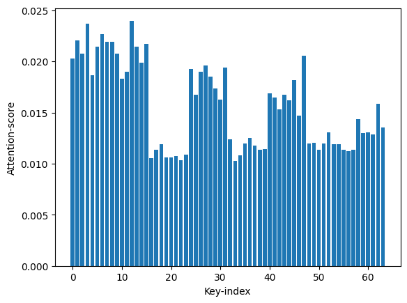
1
2
3
4
5
6
7
plt.bar(x = np.arange(len(result)), height = result)
plt.xlabel('Element-index')
plt.ylabel('Element-value')

'''
Text(0, 0.5, 'Element-value')
'''

9.5 Matrix-based implementation
1
2
3
keys_mat = np.array(keys)
values_mat = np.array(values)
queries_mat = np.array(queries)
1
2
3
4
5
6
def attentionQueryMatrix(queries, keys, values):
    norm = np.sqrt(len(keys[0]))
    attention = np.matmul(queries,keys.transpose())/norm
    attention = np.exp(attention)
    attention = attention/attention.sum(axis = 1, keepdims=True)
    return attention, np.matmul(attention,values)
9.6 Apply the function and plot the results
1
2
3
4
5
6
7
8
9
10
11
attentions, results = attentionQueryMatrix(queries_mat, keys_mat, values_mat)
plt.imshow(attentions)
plt.xlabel('Key-index')
plt.ylabel('Query-index')
plt.colorbar()
plt.show()
keys_mat.shape

'''
(64, 8)
'''
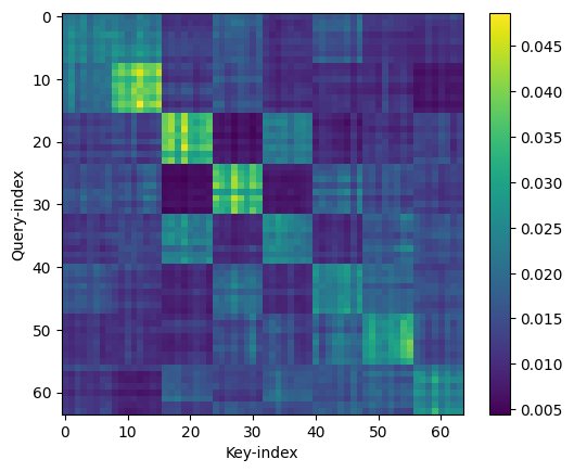
1
2
3
4
5
6
7
plt.bar(x = np.arange(len(result)), height = results[0])
plt.xlabel('Element-index')
plt.ylabel('Element-value')

'''
Text(0, 0.5, 'Element-value')
'''

1
2
3
4
attentions = np.zeros((len(keys),len(keys)))
for i in range (len(keys)):
    a, _ = attentionQuery(queries[i], keys, values)
    attentions[i,:] = a
9.7 Masked attention
1
2
3
4
5
6
7
8
def maskedAttentionQueryMatrix(queries, keys, values):
    norm = np.sqrt(len(keys[0]))
    attention = np.matmul(queries,keys.transpose())/norm
    attention = np.exp(attention)
    xs, ys = np.meshgrid(np.arange(attention.shape[1]), np.arange(attention.shape[0]))
    attention[ys<xs] = 0
    attention = attention/attention.sum(axis = 1, keepdims=True)
    return attention, np.matmul(attention,values)
9.8 Apply the masked function and plot the results
1
2
3
4
5
6
7
plt.bar(x = np.arange(len(result)), height = results[0])
plt.xlabel('Element-index')
plt.ylabel('Element-value')

'''
Text(0, 0.5, 'Element-value')
'''
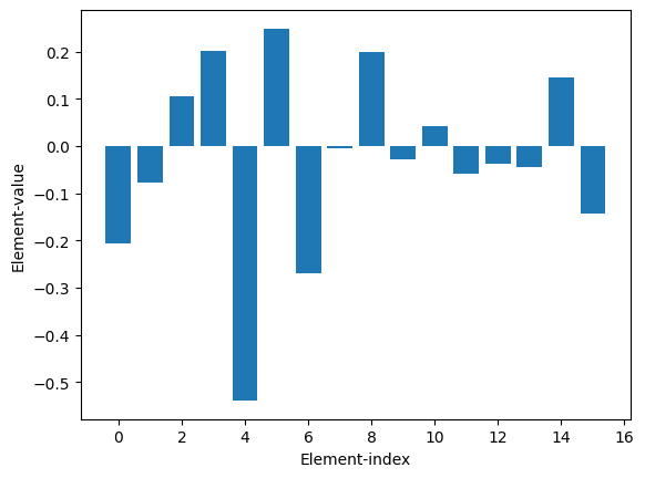
1
2
3
4
5
6
7
8
9
10
11
attentions, results = maskedAttentionQueryMatrix(queries_mat, keys_mat, values_mat)
plt.imshow(attentions)
plt.xlabel('Key-index')
plt.ylabel('Query-index')
plt.colorbar()
plt.show()
keys_mat.shape

'''
(64, 8)
'''