计算机视觉 - Computer Vision Code
计算机视觉 - Computer Vision Code
Lab 1
Introduction
基本库导入
1
2
3
4
5
6
# Imports
import skimage
import scipy
from matplotlib import pyplot as plt
import numpy as np
from utils import show_binary_image
处理图像
1
2
3
4
5
6
7
8
9
10
11
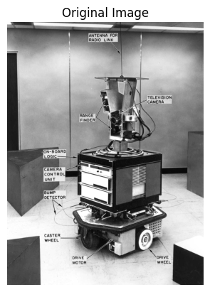
# Read image
shakey = skimage.io.imread('shakey.jpg')[:,:,0] #提取绿色通道Extract the Green Channel
# Display the image 显示图像
plt.imshow(shakey,cmap="gray")
plt.title("Original Image")
plt.axis('off')
plt.show()
print("Shakey raw values", shakey)
Outputs:
初始化算子
1
2
3
4
5
6
7
8
9
sobel_x = np.array(
    [[1,0,-1],
     [2,0,-2],
     [1,0,-1]])

sobel_y = np.array(
    [[1,2,1],
     [0,0,0],
     [-1,-2,-1]])
算子处理图片后,显示出超出阈值的部分(>50)
1
2
3
4
5
6
7
8
9
10
11
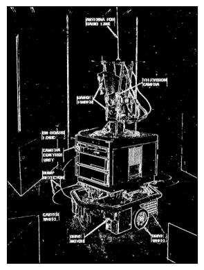
# Applying a filter
# We convert the output type to floats in order to preserve negative gradients
# We can also threshold the image using the > operator
threshold_shakey_sobel_x = abs(scipy.signal.convolve2d(shakey, sobel_x))>50
print("Boolean Thesholded Values:")
print(threshold_shakey_sobel_x)
# Here we use the binary helper function as our image is now binary
print("Boolean Thesholded Image:")
show_binary_image(threshold_shakey_sobel_x)
Outputs:
Task1
把经过算子x和算子y处理过的图像通过mangnitude处理成一个图像(这时不需要加threshold), 然后查看不同threshold下有何区别
1
2
3
4
5
6
7
8
9
10
11
12
13
14
15
16
17
18
19
20
21
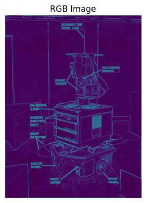
def mangnitude(x,y):
return np.sqrt(np.square(x) + np.square(y))
def show_rgb_image(image):
plt.imshow(image)
plt.title("RGB Image")
plt.axis('off')
plt.show()
shakey_sobel_x = abs(scipy.signal.convolve2d(shakey, sobel_x))
shakey_sobel_y = abs(scipy.signal.convolve2d(shakey, sobel_y))
m = mangnitude(shakey_sobel_x,shakey_sobel_y)
show_rgb_image(m)
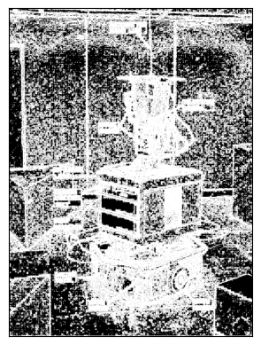
show_binary_image(m > 10)
show_binary_image(m > 50)
show_binary_image(m > 100)
Outputs:

Task 2
使用精度更小的算子处理图像,并对比差异
1
2
3
4
5
6
7
8
9
10
11
12
13
14
15
16
17
18
roberts_x = np.array(
    [[1,0],
     [0,-1]])

roberts_y = np.array(
    [[0,1],
     [-1,0]])

shakey_roberts_x = abs(scipy.signal.convolve2d(shakey, roberts_x))
shakey_roberts_y = abs(scipy.signal.convolve2d(shakey, roberts_y))

m_roberts = mangnitude(shakey_roberts_x,shakey_roberts_y)

show_rgb_image(m_roberts)

show_binary_image(m > 50)

show_binary_image(m_roberts > 50)
Outputs:
Task 3
用近似mangnitude的方法处理,对比哪个效果更好
1
2
3
4
5
6
7
8
9
10
def mangnitude_appr(x,y):
    return np.abs(x) + np.abs(y)

m_appr = mangnitude_appr(shakey_sobel_x,shakey_sobel_y)

show_rgb_image(m_appr)

show_binary_image(m > 40)

show_binary_image(m_appr > 40)
Outputs:

Lab 2
Task 1
1
2
3
4
5
6
7
8
9
10
11
12
13
14
15
16
17
18
19
20
21
shakey = skimage.io.imread("shakey.jpg")[:,:,0] #取出绿色通道

# 分别应用高斯3x3与高斯5x5

gaussian_3x3_result = scipy.signal.convolve2d(shakey, gaussian_filter_3x3)

gaussian_5x5_result = scipy.signal.convolve2d(shakey, gaussian_filter_5x5)

show_binary_image(gaussian_3x3_result)

show_binary_image(gaussian_5x5_result)

# 以30为阈值处理并展示binary image

gaussian_3x3_result = scipy.signal.convolve2d(shakey, gaussian_filter_3x3)<30

gaussian_5x5_result = scipy.signal.convolve2d(shakey, gaussian_filter_5x5)<30

show_binary_image(gaussian_3x3_result)

show_binary_image(gaussian_5x5_result)
Outputs:


3x3能够保留文字
Task 2
1
2
3
4
5
6
7
8
9
10
11
12
13
14
15
16
17

std_dev = 1
mean = 0
vec = np.arange(-4, 5, 1, dtype=np.float32)

one_d_gaussian = sample_gaussian(std_dev, mean, vec)

gaussian_filter_9x9 = np.outer(one_d_gaussian, one_d_gaussian.T)

gaussian_9x9_result = scipy.signal.convolve2d(shakey, gaussian_filter_9x9)

show_binary_image(gaussian_9x9_result)

gaussian_9x9_result = scipy.signal.convolve2d(shakey, gaussian_filter_9x9)<30

show_binary_image(gaussian_9x9_result)
Outputs:
Task 3
1
2
3
4
5
6
7
8
9
10
11
12
13
start_time_1d = time.monotonic()
scipy.signal.convolve(shakey, one_d_gaussian)
end_time_1d = time.monotonic()

start_time_2d = time.monotonic()
scipy.signal.convolve2d(shakey, gaussian_filter_9x9)
end_time_2d = time.monotonic()

cpu_time_1d = end_time_1d - start_time_1d
cpu_time_2d = end_time_2d - start_time_2d

print(cpu_time_1d)
print(cpu_time_2d)
Outputs:
0.030999999988125637
0.1880000000091968
Task 4
使用laplacian算子,查看边缘检测结果是否更好/更差
1
2
3
4
5
6
7
8
9
10
11

laplacian_filter = np.array([[1, 1, 1],
                             [1, -8, 1],
                             [1, 1, 1]])

laplacian_result = scipy.signal.convolve2d(shakey, laplacian_filter)

edges = zero_cross(laplacian_result)

show_binary_image(edges)
Outputs:
Task 5
本文由作者按照 CC BY 4.0 进行授权